Efficient Entity Resolution with MFIBlocks

Efficient Entity Resolution with MFIBlocks Batya Kenig, Avigdor Gal Technion-Israel Institute of Technology

{batyak@tx,avigal@ie}.technion.ac.il

ABSTRACT Entity resolution is the process of discovering groups of tuples that correspond to the same real world entity. In order to avoid the prohibitively expensive comparison of all pairs of tuples, blocking algorithms separate the tuples into blocks which are highly likely to contain matching pairs. Tuning is a major challenge in the blocking process. In particular, contemporary blocking algorithms need to provide a blocking key, based on which tuples are assigned to blocks. Due to the tuning complexity, blocking keys are manually designed by domain experts. In this work, we introduce a blocking approach that avoids selecting a blocking key altogether, relieving the user from this difficult task. The approach is based on maximal frequent itemsets selection. This approach also allows early evaluation of block quality based on the overall commonality of its members. A unique feature of the proposed algorithm is the use of prior knowledge of the estimated sizes of duplicate sets in enhancing the blocking accuracy. We report on a thorough empirical analysis, using common benchmarks of both real-world and synthetic datasets which exhibit the efficiency of our approach.

Keywords Entity Resolution, Frequent Itemsets, Blocking

1. INTRODUCTION Entity resolution is a fundamental problem in data integration, an area that deals with various aspects of combining data from different sources. Entity resolution refers to the problem of determining which tuples (using relational notation) resolve to the same real-world entity. At the heart of the entity resolution process is the challenge to match tuples that share no unique identifiers, may come from non-matching schemata, and may consist of typos, outof-date information, and missing information. Entity resolution algorithms typically compare the content of attributes or tuples to determine if they match and merge matching tuples into one. Such a comparison may be prohibitive for big data sets if all tuple pairs are compared and hence pairwise comparison is typically preceded Permission to copy without fee all or part of this material is granted provided that the copies are not made or distributed for direct commercial advantage, the VLDB copyright notice and the title of the publication and its date appear, and notice is given that copying is by permission of the Very Large Data Base Endowment. To copy otherwise, or to republish, to post on servers or to redistribute to lists, requires a fee and/or special permission from the publisher, ACM. VLDB ‘09, August 24-28, 2009, Lyon, France Copyright 2009 VLDB Endowment, ACM 000-0-00000-000-0/00/00.

by a blocking phase, a procedure that divides tuples into mutually exclusive subsets (blocks). Tuples assigned to the same block are ideally resolved to the same real-world entity. In practice, tuples in a block are all candidates for the more rigorous tuple pair-wise comparison. Therefore, blocking algorithms should be designed to produce quality blocks, containing as many tuple matches and avoiding as many non-matches as possible. Therefore, the size of the generated blocks should not be too small, to avoid false negatives, or too large, to avoid false positives. Larger blocks also increase the time spent of pair-wise tuple comparison and hence, blocking algorithms aim at balancing the need to reduce false negatives and the need to reduce performance overhead. Several blocking algorithms were proposed in the literature, including Sorted Neighborhood [1], Canopy Clustering [2] and Qgram indexing [3]. In this work we offer a novel blocking algorithm, MFIBlocks, that is based on iteratively applying an algorithm for mining Maximal Frequent Itemsets [4]. MFIBlocks offers two major unique features. Firstly, MFIBlocks waves the need to design a blocking key. A blocking key in blocking algorithms is taken as the value of one or more of a tuple’s attributes. Blocking keys have to be carefully designed, to avoid false negatives by assigning matching tuples to different blocks. Therefore, attributes in the blocking key should contain few errors and missing values and the design of a blocking key should take into account the frequency distribution of values in the attributes of the blocking key to balance the block sizes. MFIBlocks relieves the designer from the difficult task of constructing a blocking key by effectively choosing a key automatically, based on the data at hand. This feature supports an efficient handling of typos, missing information, and uncertain schema matching. MFIBlocks also allows a dynamic and flexible choice of a blocking key, so that different blocks can be created based on different keys. This approach is in line with the state-of-the-art in clustering literature (see, e.g., [5]) and extends the current conception of a single-key-fits-all. MFIBlocks is designed to discover entity sets with largely varying diverse sizes. By discovering clusters with the largest possible commonality, the resulting entity sets enable clustering tuples in decreasing cluster sizes according to the expected sizes of duplicate entity sets in the input. These sets capture the commonality of their support sets and therefore enable the evaluation of blocks by generalizing known similarity metrics for string comparison. Also, MFIBlocks can effectively utilize a-priori knowledge of expected sizes of entity sets. Finally, MFIBlocks creates blocks that are compact set (CS) and in sparse neighborhood (SN), in accordance with the principles identified in [6]. As such, local structural properties of the dataset

tuples

Database D

Blocking candidate pairs

Tuple pair comparison candidate pair + similarity measure + threshold

Classification

Match

Non-Match

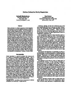
Figure 1: Entity resolution process are used during the discovery and evaluation of tuple clusters. This paper introduces the MFIBlocks algorithm, discusses its properties, and perform a thorough empirical analysis, demonstrating its superiority to existing blocking algorithms. The rest of the paper is organized as follows. Section 2 overviews related work and preliminaries. The entity resolution model is introduced in Section 3. Then the algorithm and its various design issues are discussed in Section 4. In Section 5 we provide an empirical analysis over several benchmark datasets. We conclude in Section 6 with a summary and a discussion of future work.

2. BACKGROUND The general, unsupervised entity resolution process illustrated in Figure 1 has a blocking, comparison and classification stage. In some cases a standardization process will precede these steps in order to raise the process effectiveness. The output of the blocking stage are blocks where each pair of tuples in a block is considered as a candidate pair. Only candidate pairs are then compared using more sophisticated comparison functions (see below). Pairs of tuples that were pruned by the blocking process are automatically classified as non-matches. Using one or more similarity measures such as the Jaccard coefficient [7], edit distance or the Jaro-Winkler method [8], an entity resolution framework will use the similarity to classify a candidate pair of tuples as matching or non-matching. The tuple pair (t1 , t2 ) is represented as a vector v = [v1 , ..., vk ] with k components corresponding to the k comparable attributes of the pair. Each vi shows the similarity of the ith field for the tuple pair, in most cases the entries in the vector v are in the range [0, 1]. A function f over the values of these entries will be used to classify a pair as a match or non-match according to a predefined threshold. In this paper we focus on the blocking stage. The algorithm proposed returns overlapping clusters, namely, a tuple may belong to more than one cluster. An ER algorithm, on the other hand, returns a partition of the database such that the members of each partition correspond to a common entity. Section 2.1 provides a brief overview of known blocking algorithms, positioning our work on this background. An in-depth theoretical and experimental survey of the current blocking techniques is available in [9]. Section 2.2 overviews the concept of frequent and maximal frequent itemsets.

2.1 Related Work All blocking techniques described in this section require the definition of a blocking key which is orthogonal to the selection of the blocking algorithm. Furthermore, this key is global in the sense that the clusters returned by the blocking algorithm are derived based on similarity only over this specific key. All blocking techniques except for Standard blocking, which has been used as a pruning step for ER algorithms since its beginning [10], create overlapping blocks. This means that a tuple may belong

to more than a single block and will ultimately be compared with all tuples which share a block with it. Most blocking methods are implemented using an inverted index structure [9]. The blocking key value for each tuple is transformed to a set of keys in the index structure which are later used to extract the blocks a certain tuple belongs to. Q-gram indexing, also known as fuzzy blocking is implemented in the FEBRL [11] record linkage system. The blocking key values are converted into a list of q-grams and sub-lists of all possible combinations of the q-grams are built according to a configured threshold in the range [0, 1]. The q-grams in the resulting sublists are concatenated and inserted as keys into an inverted index, which is used to retrieve sets of tuples in a block. In suffix array based blocking [12] an inverted index is built from the blocking key values and their suffixes. A tuple identifier will be inserted into several blocks according to the length of its blocking key value. In order to limit the maximum block size, only blocks containing less than a certain number of tuple identifiers are considered. Canopies [2] are overlapping blocks created by applying a cheap comparison metric to tuples. Canopy clusters are generated by randomly selecting a tuple from a pool, and adding close tuples to the cluster. Of these tuples, all tuples within a tighter similarity threshold are removed from the candidate pool of tuples. This process is repeated until no candidate tuples are left. In the Sorted Neighborhood [1] approach, a key is extracted from each tuple by computing its blocking key value. The tuples are then sorted according to this key and a fixed-size window is moved through the sorted list of tuples. Only tuples that fall into the same window are compared, thus limiting the number of comparisons. The effectiveness of this approach is dependent upon the comparison key selected in the first step. This procedure can be carried out multiple times, each time with a different key in order to reach a satisfactory recall level. The String-Map based indexing technique [13] is based on mapping the blocking key values to points in a multi-dimensional space such that the distances between pairs of strings are preserved. A d-dimensional grid-based inverted index is then constructed. The coordinate values of the points in each one of the dimensions act as the keys to the index. All tuple identifiers whose corresponding tuple was mapped to a point whose value in a certain dimension belongs to the same cell are inserted into the same inverted index list. All blocking methods discussed so far rely on a careful construction of a blocking key in order to index or sort the database tuples. This blocking key composition requires not only knowledge of the distribution and error characteristics of the data, but also requires a crisp correspondences between attributes in the two sources. [14] offer a learning method to automatically select the best blocking key, by applying the approximation algorithm to the set cover problem. In this setting, the elements to be covered are the matching pairs of tuples while the sets’ weights are the number of false negative pairs they cover. MFIBlocks, on the other hand, makes do with the need to configure a blocking key. Instead, the algorithm allows all attribute values to participate in the clustering criteria. Using itemset mining, MFIBlocks does not perform any attribute-specific indexing or comparison. Therefore, it gracefully handles uncertain correspondences between attributes. Many of the blocking techniques discussed employ a limit parameter on the size of the blocks which may be created. This is done in order to avoid the cost of having to compare many candidate pairs which results when large blocks are generated. This parameter may be difficult to come-by and as opposed to the proposed

approach has no relation to the expected sizes of tuple-clusters which refer to the same entity.

2.2 Frequent Itemsets We now provide background on mining frequent itemsets [15], as a basis for the proposed algorithm. ⟨ Let M = {I⟩1 , I2 , . . . , Im } be a set of items. Let D = T 1 , T 2 , · · · , Tn

be a database of transactions, where Ti =

(tid, I) is a transaction with identifier tid which contains a set of items I such that I ⊆ M . The support of a set of items, I ⊆ M , is the set of transactions in D that contain I. tid 1 2 3 4 5

A a1 a1 a2 a2 a1

B b1 b1 b2 b2 b3

C c1 c2 c3 c2 c4

Table 1: Sample Transaction Database

Example Table 1 contains five transactions with the items M = {a1 , a2 , b1 , b2 , b3 , c1 , c2 , c3 , c4 }. Transaction 1 support items {a1 , b1 , c2 }. The support set of itemset {a1 , b1 } = {t1 , t2 }. I is frequent if I’s support size is no less than a minimum support threshold min sup. A useful observation, called the downward closure property, is that any subset of a frequent itemset is also a frequent itemset [15] and therefore a frequent itemset cannot contain an infrequent itemset. Given a transaction database D and a minimum support threshold min sup, the problem of finding the complete set of frequent itemsets (FI) is called the frequent itemset mining problem. A major challenge in mining frequent itemsets from a large or dense (contains a large amount of different items) dataset, is that a too low min sup thresholds generates a huge number of frequent itemsets. For example, if there is a frequent itemset of size l, then all 2l − 1 nonempty subsets of that itemset are also frequent due to the download closure property. To overcome this difficulty, we introduce next maximal frequent itemsets (MFIs for short) [16]. A frequent itemset X is called maximal if there does not exist a frequent itemset Y such that Y ⊃ X. Due to the downward closure property of frequent itemsets, all subsets of maximal frequent itemsets (MFIs) are frequent, while all supersets of such items are infrequent. Example There are 7 frequent itemsets from Table 1, with min sup = 2: {{a1 }, {a2 }, {b1 }, {b2 }, {c2 }, {a1 , b1 }, {a2 , b2 }}. and 3 maximal frequent itemsets with the same support are: {{a1 , b1 }, {a2 , b2 }, {c2 }}. The MFI mining algorithm we use is FPMax [4], which received the best implementation award and displayed the best performance for both low and high supports in the frequent itemset mining implementations report from 2003 [17].

3. MODEL Consider a relation R (A) and an instance of R, D. An entity resolution algorithm partitions D into P , representing groups of the same real world entity. As a first step towards constructing P ,

a blocking algorithm is used to reduce the number of comparisons among tuples. Tuples are placed in possibly more than one block from B = {b1 . . . bm }, referred to as MFI-blocks, of size at least minsup. fB : D → B maps a tuple t ∈ D to zero or more blocks in B. Two tuples, t, s ∈ D will be compared in an entity resolution algorithm if and only if fB (t) ∩ fB (s) ̸= ∅. A block b = {t1 , . . . tl } ∈ B corresponds to an MFI bI = {i1 , . . . ik }. The values i1 , . . . ik are shared by all tuples t1 , . . . , tl ∈ b. Each MFI block b ∈ B is mapped to a value in the range [0, 1] using some score function σ (discussed in Section 4.2) that captures the similarity or commonality among tuples in a block. We assume that the score function is monotonic with respect to the itemset containment. That is, for two itemsets bI1 ⊇ bI2 with corresponding support blocks b1 , b2 , σ(b1 ) ≥ σ(b2 ). The score function may be computed on tuples as a whole or on a subset of the attributes. When the score function is confined only to the values of a subset of attributes Ai , we denote this by σi . The Compact Set (CS) and Sparse Neighborhood (SN) criteria [6] are useful for characterizing “good” entity resolution clusters, and thus are also desired properties of blocks returned by a blocking algorithm. Therefore, we adapt these principles for blocking algorithms, as follows. D EFINITION 1. Let Ai ⊆ A be a subset of attributes. An Ai CS is a set of tuples such that for every two tuples t1 , t2 ∈ Ai -CS, σi (t1 , t2 ) > σi (t1 , t3 ) where t3 ̸∈ Ai -CS. The CS definition of [6] is altered to consider a general score function rather than distance between tuples. Whenever score is interpreted as distance, the two criteria converge. In the MFIBlocks algorithm, tuples are grouped together into a block b based on a common set of items bI , originating from some set of attributes Ai ⊆ A. We can therefore state the following proposition. P ROPOSITION 3.1. Let bI be an MFI with items originating from the values of attributes Ai ⊆ A, with corresponding supportblock b. The tuples in b form an Ai -CS. P ROOF. Consider tuples t1 , t2 ∈ b and assume, by contradiction, that there is a tuple t3 ̸∈ b, such that σi (t1 , t3 ) > σi (t1 , t2 ). In this case, t3 must have at least the same commonality, over Ai values, with t1 as does t2 , therefore t3 must support bI , contradicting our assumption that t3 ̸∈ b. D EFINITION 2. The neighborhood of a tuple t is a set of tuples that share some block with t: ∪ N (t) = b. b∈fB (t)

The neighborhood growth (NG) of tuple t is the cardinality of N (t), N G(t) = |N (t)|. Higher N G(t) reflects a higher number of pairwise comparisons for tuple t in the entity resolution process. Our definition of Sparse Neighborhood (SN) therefore considers N G(t) and the minimal block size minsup. D EFINITION 3. A set of tuples D′ ⊆ D is considered a sparse neighborhood, denoted SN (agg, p), if |D′ | = 1 or aggt∈D′ N G(t) ≤ p · minsup where p > 1 is a predefined constant.

Block# b1 b2 b3 b4 b5 b6 b7

Participants {t4 , t5 , t6 } {t4 , t5 , t8 } {t3 , t4 , t8 } {t3 , t4 , t6 , t7 } {t4 , t5 , t7 } {t9 , t10 , t11 } {t10 , t11 , t12 }

Itemset {savannah, tuthill place, 0752913455} {humphreys, 0752913455} {4120, 0752913455} {nsw, 0752913455} {0752913455, 3050536} {elwood, nsw, 19920405, 0727375124} {nsw, 21, 0727375124}

Table 2: MFIs of the Case Study

The aggregate function we use in the proposed algorithm is max. According to Definition 3, to maintain a clustering which complies to the sparse neighborhood condition, all blocks with tuples whose neighborhood growth is larger than p · minsup should be rejected. We will denote by Bo the set of blocks returned by the algorithm. A threshold mint h is used to determine the minimal score of output blocks. Only blocks b ∈ B for which σ(b) ≥ mint h may potentially be included in Bo . A tuple which, upon termination of the blocking algorithm, belongs to at least one block b ∈ Bo with size equal or greater than i (|b| ≥ i), will be considered i-covered. This means that if a tuple t belongs to a block b ∈ Bo that corresponds to the MFI bI discovered while executing the MFI algorithm with support minsup, then t is minsup-covered. Tuples that do not belong to any b ∈ Bo are considered not to have a match and remain a singleton. Example Table 2 presents the maximal frequent itemsets mined from the case study (Table 3) with minsup = 3. The items in b1 originate from attributes ‘given name’, ‘address1’, and ‘phone’ while the items in b2 originate from attributes ‘surname’ and ‘phone’. Assume the use of the Jaccard similarity measure [18] is used as the score function. Then, σ(t4 , t5 , t6 ) = 38 and σ(t9 , t10 , t11 ) = 84 . The sets in B are all Ai -CS. For example, there is no tuple closer to t4 over attributes ‘given name’, ‘address1’, and ‘phone’ than t5 and t6 . Likewise, there is no tuple closer to t4 over attributes ‘postcode’ and ‘phone’ than t3 and t8 . Also, for p = 2 the generated block set complies with the SN criterion, maxt∈D N G(t) = N G(t4 ) = 5 ≤ 2 · minsup = 6. Finally, the tuples t3 -t12 are 3-covered, while each of tuples t1 , t2 , t13 , t14 remains a singleton.

4. THE MFIBLOCKS ALGORITHM This section introduces MFIBlocks in a modular fashion. We start with describing the data setup (Section 4.1) followed by a method for assessing cluster quality in Section 4.2. We then discuss the selection of minsup (Section 4.3) and the application of the compact set and sparse neighborhood criteria (Section 4.4). The algorithm pseudo-code is presented in Section 4.5, together with an analysis of its formal properties. To illustrate the various elements of the algorithm, we use a running case study, given in Table 3. This example has five entities, three of which have multiple tupes of various sizes (6,4 and 2). The tuples in Table 3 were generated using the database generator of FEBRL [11].

nah’ for the surname attribute while the same value appears under the first name attribute in tuple t4 . We would like to maintain this difference after transforming it into a transaction data set. Also, we would like to provide support for overcoming variations that stem from abbreviations, synonyms, and typographical errors. For example, we would like to avoid considering the terms ’Marta’ and ’Martha’ as totally different items by the algorithm regardless of their obvious similarity. As a first step, a lexicon of items is created and enumerated. Each attribute value is separated into q-grams, a known approach in Information Retrieval for overcoming typographical errors. Identical q-grams, originating from matching attributes, receive the same id. q-grams that originate from non-matched attributes are assigned different ids even if they are identical. Once the lexicon is constructed, database tuples are transformed into a transaction database by replacing attribute values with the ids of their corresponding q-grams. At this point, a tuple t becomes a bag of items, referred to as t.items, where each item id, id ∈ t.items corresponds to a q-gram in t. Each q-gram (identified by its id) is associated with a relative weight indicating the quality (in case of a probabilistic schema matching [19, 20]) and discriminative power of the attribute from which the q-gram originates. This value is used to asses the quality of a block whose corresponding MFI contains the specified qgram.

4.2

Assessing block quality

A block represents some commonality among its member tuples. We now aim at evaluating the quality of a block in terms of this commonality. Poor quality may be a result of a small size of a block, meaning that only a few items share the block commonality. Another problem may be that the items in a block originate from low quality attributes, containing inaccurate and missing values. The tuples in a block may share items of limited discriminative power, e.g., a certain item may appear in half of the transactions. Finally, the differences between tuples may surpass the commonality represented by the block. To asses the quality of a block we use a version of the extended Jaccard similarity [18], comparing a set of similar tokens (rather than only two tokens with the common Jaccard similarity). Let b be a block representing a maximal frequent itemset bI . The group of items in b is Mb = ∪t∈b t.items, where t.items represents the q-grams of tuple t. This set can be divided into three disjoint groups. First, the set of common items, denoted Cb , is the set of items that are present in each and every tuple t ∈ b. This set of items is actually the maximal frequent itemset bI . The second set is the set of near items, denoted Lb , consisting of items that appear in one of their abbreviations in nearly all t ∈ b. In order for an item i to be considered near, the following must hold: 1 ∑ αb (i) = max Sim(j, i) ≥ sim th j∈t.items |b| t∈b

4.1 Data setup

where sim th is a configured similarity threshold and the similarity measure we used is the Jaro-Winkler method [21]. Finally, the set of uncommon items, denoted Ub , consists of items that neither common or near. Intuitively, these appear in only a small fraction of the tuples in b.

Frequent itemset mining algorithms run on a data set of transactions t ∈ D, where each transaction is composed of a set of items I. We now describe a method for transforming a database into a suitable input data set for the MFI algorithm. In this preparation phase we would like to maintain the structural information of the data. For example, tuple t3 in Table 3 contains the value ‘savan-

Example In a block b = {t1 , t2 } from Table 3, the q-grams originating from values from all attributes except ‘address1’, ‘suburb’ and ‘age’ are identical, and will be classified as common items. The q-gram ‘mur’, for instance, originating from t1 ’s ‘suburb’ attribute will be classified as a near item because it is relatively

index 1 2 3 4 5 6 7 8 9 10 11 12 13 14

given name xavier xavier savannah savannah savannah savannah savanmwh savanah chelsear chelara chelsea chelsibe raquel annabel

surname tomich tomich savannah humphreys humphreys humphfjfeys humpmhheys humphreys hanns hanna hanna habmy rudad burleigh

address1 gamban square gambandsquare tuthiolzlace tuthill place tuthill place tuthill place tuthill place tuthill klace mugglestoea mugglestonna mugglestone mugglestone wilkinsfateet wakelin circuit

suburb murgon mudrgon dayle sford daylesford daylqogrd daylesord daylesford dayles fofrd elwood elwood elwood elwood wellington point newborough

postcode 2150 2151 4120 4120 4102 4219 4105 4120 2119 2161 2117 2117 4054 2150

state

nsw nsw ndw nsw nsw nhs nsw nsw nsw nsw sa nsw

birthday 19240904 19240904 19680729

age 36 37

19920405 19920405 19920405 19907715 19551226 19150311

92 21 21 21 36 30

phone number

0752913455 0752913455 0752913455 0752913455 0752913455 0752913455 0727375124 0727375124 0727375124 0727375124 0743902126 02 48546447

socSecId 2432656 2432656 3005536 3050536 3050536 3050586 3050536 3099036 1594344 1592943 1594343 1594353 1770634 5862603

Table 3: Running example

close to the q-gram ‘mud’ originating from t2 ’s ‘suburb’ attribute (Sim(‘mud′ , ‘mur′ ) ≥ 0.9). Therefore we can say that an abbreviation of ‘mur’ appears in all tuples in the block. The values in the ‘age’ attribute will be classified as uncommon. Intuitively, we would like to give a higher score to clusters containing many common or near items and a few uncommon items. We propose to set a score using the tf/idf weighting scheme [22], a common measure in Information Retrieval. The tf/idf score of an item i in itemset bI with support b is computed as follows: vb (i) = log(tfb (i) + 1) · log(idfb (i)), where tfb (i) is the number of times item i appears in b (if item i ∈ bI then tfb (i) ≥ |b| ). idfb (i) = |D| where ni is the number ni of tuples in database D that contain item i. The tf/idf weight for an item i in itemset bI is high if i appears a large number of times in the block b (large tfb (i) ) and i is a sufficiently rare item in the database (large idfb (i)). The above score may be calculated for all items in M . As discussed in Section 4.1, the user may add metadata to the ids representing items through the lexicon. This metadata may include relative weights indicating the quality and discriminative power of the attributes from which the items originated. We will represent the weight of item i ∈ bI as w(i). Combining the tf/idf score and item weights in the extended Jaccard similarity function [18] results in the following score function: ∑ Jaccard(b) =

i∈Cb

w(i)vb (i) + ∑

∑ i∈Lb

w(i)vb (i) · αb (i)

i∈Mb w(i)vb (i)

(1) The common item set, Cb , is discovered by the MFI mining algorithm. The question that remains to be answered is how to find all of the near items. Since we assume that an item i ∈ L is such that either it or its abbreviation is in almost all of the tuples in the support set, we may choose a tuple t ∈ b at random and run over its items. If an abbreviation of item i ∈ t.items appears in nearly all records in b, then we may classify i as a near item. This makes the discovery of near items efficient since we iterate only over items in a single tuple for each block. The distance metric used to measure the distance between items is the Jaro-Winkler [8] metric. It is important to note that had we classified the items in b’s tuples to only common and uncommon items, we would have underestimated the commonality of b’s tuples. The reason is that the tf/idf scores of the near items would have been considered as uncommon in the score function (Eq. 1). This would have drastically lowered the score such that it would not be able to reflect the actual commonality

among the tuples in b.

4.3

Selection of minsup

As explained in Section 2.2, the MFI mining algorithm receives minsup as a parameter indicating the minimum size of the MFI’s support set or minimal block size. The selection of minsup is highly important in the context of MFI-based blocking. The minsup parameter should be set to the expected size of the duplicate clusters in the database. In many scenarios this value may be known in advance, for example, if we know that the tuples in a certain database originated from two clean sources, then we may assume that each tuple may have at most a single duplicate and we will set the minsup parameter to 2. This will lead to the mining of maximal frequent itemsets that are supported by at least two tuples. If minsup is set too high then either no maximal frequent itemsets will be mined, because there will not be any commonality among clusters of a large size. Another scenario is that large clusters will have some commonality, but since it may be small or insignificant, their score will not pass the minimum threshold. On the other hand, if minsup is set too low, then there is a chance that the larger clusters will be missed, resulting in lower recall. The reason this may happen is that inside the larger cluster there could be groups of records with higher commonality, causing the generation of larger MFIs with a smaller support size. Since our algorithm mines only maximal frequent itemsets, the itemset that captures the commonality of the larger cluster will not be returned by the mining algorithm. In order to alleviate these issues, the minsup parameter should be large enough so that the larger duplicate clusters will not be missed. For example, in the running example in Table 3, if we run the algorithm with a minsup = 2 then the cluster containing tuples 38 would have been missed. The reason is that tuples 4 and 5 have a larger commonality than other tuples in the set 3-8 because they are identical in attributes ‘given name’, ‘surname’, ‘address’, ‘phone’ and ‘social security id’. This is not the case for all the tuples in this set. In many cases the duplicate clusters in the database are not of uniform size. In the running example in Table 3, there are duplicate clusters of sizes 6, 4 and 2. Under our assumption, duplicate clusters (of any size) should have a high commonality and will therefore receive a high value by the scoring function (Eq. 1). We also assume that the commonality (MFI) is unique to the duplicate cluster, thus only records which belong to the duplicate cluster (i.e, refer to the same entity), will support its corresponding MFI. Therefore, if we run the MFI algorithm with minsup = 6, then high scoring blocks (of size at least 6) are of high commonality and are therefore good candidates to search in for matching pairs. When running the

MFI algorithm with minsup = 6, the MFIs corresponding to the size-4 and size-2 clusters will not be returned by the MFI algorithm due to lack of support. After the size-6 clusters are discovered using the MFI mining algorithm, we can delete from the database all of the 6-covered records, and rerun the MFI mining algorithm on the remaining records (records 1-2,9-12). This time the MFI mining algorithm will run with minsup = 4 and discover duplicate clusters of size 4 (records 9-12). After this, the algorithm may be rerun on the leftover records 1-2 with minsup = 2 to discover the size-2 block.

4.4 Applying the SN and CS criteria We have already established that blockings B = {b1 . . . bm } which comply with the SN criterion [6] have desirable properties. Another advantage in applying the SN criterion, as described in Section 3, is further ease of configuring the algorithm. The score threshold parameter has a dramatic affect on the quality of the blocking returned by the MFIBlocks algorithm. A threshold set too low will lead to low precision while a threshold set too high will bring to a decrease in recall. In most cases, the threshold is highly dependent on the error characteristics of the data. The configuration of the SN criterion is simpler as it places a limit on a tuple’s neighborhood based on the expected size of the clusters. For example, if we are expecting clusters of size 2, we may decide to limit the neighborhood of each tuple to a size 4 or 6, by setting the parameter p to 2 or 3 respectively. Therefore, the algorithm will search for a threshold th, larger than some absolute minimum threshold min th, such that when blocks b whose score is below this threshold th, i.e, score(b) < th are eliminated, the reduced blocking satisfies the SN criterion (i.e, maxt∈D N G(t) < p · minsup). It could be that under no circumstances can the NG criterion be satisfied for a certain minsup. In such a case the search for threshold th will return 1, and we can deduce that no blocking exists that will satisfy the NG criterion. For example, if we have a database with three identical tuples, and the MFI mining algorithm has been applied with minsup = 2 then exactly one block containing all three tuples will be created, and since the tuples are identical, its score will be 1. Setting an NG limit of p = 1 will cause this blocking to be rejected since every tuple has a neighborhood of size 3. Increasing the min threshold is not possible as it has reached the maximum. The example below illustrates the process described: Example Let us look at a database built up of tuples t1 , t2 , t13 , t14 from Table 3. Duplicate tuples t1 and t2 are relatively close and would receive a high score by the similarity function. An administrator, not aware of the quality or commonality of duplicate tuples, may not know to set the threshold to a high value (> 0.5). If we run the MFI mining algorithm with minsup = 2 on the database of tuples D = {t1 , t2 , t13 , t14 } from Table 3 with a minimum threshold set to 0, we will get the following blocks (Near items do not appear in the MFIs for simplicity): B = {b1 = {t1 , t2 },b2 = {t1 , t14 }, b3 = {t1 , t13 }}, with corresponding itemsets BI = {bI1 = {xavier, tomich, 19240904, 2432656}, bI2 = {2150}, bI3 = {36}} In this scenario, setting the N G limit to exactly the size of the expected cluster sizes, i.e, maxt∈D N G(t) ≤ p · minsup = 1 · 2 = 2 will cause the rejection of the above blocking because N G(t1 ) =

4 > 2. As a result, the blocking will be reduced so that the SN criterion is satisfied. Since score(b1 ) > score(b2 ) and score(b1 ) > score(b3 ), the blocking will eventually reduce to B = {b1 }. By setting the N G limit to exactly the size of the expected cluster sizes (i.e, p = 1), we enabled the formation of high quality clusters even when the minimum threshold is set low. Configuring the p parameter of the NG constraint is much easier than configuring an appropriate blocking threshold. In the Experiments section (Section 5) we will show that in most cases a value p ∈ [2, 5] gives satisfactory results. The Ai − CS proposition, proved in Section 3, which states that a support block b ∈ Bo of MFI bI forms an Ai − CS, is true only when the attribute values are directly translated to items, without being tokenized. tid 1 2 3

N ame Jon Smith John H. Smith John Smit

Table 4: Name Database For example, for the database in Table 4 which contains a single “name” attribute. Had we tokanized the values in the tuples, then MFIs with minsup = 2 would be: B = {b1 = {t1 , t2 },b2 = {t2 , t3 }} with corresponding itemsets BI = {bI1 = {Smith}, bI2 = {John}} According to the Ai − CS proposition, scorename (t1 , t2 ) > scorename (t2 , t3 ) which is not necessarily true. In general, this situation can occur when a tuple t ∈ D supports different MFIs: bI1 , bI2 , both of which originate from the same set of attributes A1 ⊆ A. When working with q − gram based items, the items in bI1 , bI2 will usually have a high overlap inducing a high overlap between the corresponding blocks b1 , b2 , therefore the affect on recall is minimal.

4.5

The MFIBlocks algorithm

We now present MFIBlocks, an MFI-based blocking algorithm. The pseudo-code is detailed in algorithm 1. The algorithm receives as input the tuple database, D, an absolute minimum score threshold min th, above which the support set of an MFI will be considered as a block to search in for matching pairs and the parameter specifying the SN criterion, p. The initial support minsup is set to the size of the largest duplicate cluster expected in D. The algorithm runs in iterations, in each iteration the MFI mining algorithm is run with a smaller minimum support. The decrease in the minimum support is specified by the st parameter. Each such MFI run creates a blocking B. Tuples belonging to a cluster in a blocking that complies with the SN and minimum threshold criteria, are considered minsup-covered. The algorithm continues until either all the records in D are covered or minsup falls below 2. In each iteration the MFI mining algorithm FPMax [] FPMaxis run on the set of uncovered records (line 4). As the minsup provided to the MFI mining algorithm decreases the number of possible MFIs grows, increasing the runtime of the mining algorithm. Therefore, there is a clear advantage to first mine the larger clusters thus reducing the size of the datasets on which the more expensive iterations, with a smaller minsup, are executed.

After the MFI mining step, the clusters corresponding to each MFI returned by the algorithm are extracted and their score calculated (line 6). As described earlier, the metric used to asses the cluster is a version of the extended Jaccard similarity [18] (see Eq. 1). The MFI blocks which pass the threshold min th are added to the output set Bo . The algorithm then performs a binary search for the lowest threshold th ≥ min th such that the resulting blocking: Bo = Bo \ {b : score(b) < th}, satisfies the NG constraint (i.e, maxt∈D N G(t) ≤ p · minsup). The tuples which belong to a block b in the finalized blocking Bo are added to the set of covered records E. It is important to note that Algorithm 1 may be easily adjusted to run on any encoding of the database, including phonetic schemes such as Soundex. This type of encoding may replace the encoding of the attribute values to q-gram ids as described previously. Algorithm 1: MFI based blocking Input: Database D; minimum threshold min th; initial support size minsup; NG limit p; step st for decreasing minsup; Output: Clusters of records Bo which will be used as input to an Entity Resolution algorithm 1: Bo = ∅ {the current set of blocks} 2: E = ∅ {currently covered records in D} {repeat until all records are covered or minsup falls below 2} 3: while (E ̸= D AN D minsup ≥ 2) do 4: candidateBlocks ← M F I(D\E, minsup) {run the MFI algorithm on the uncovered tuples} 5: for all cB ∈ candidateBlocks do 6: if (Jaccard(cB) ≥ min th) then 7: Bo ← Bo ∪ cB {add as a block to the output set} 8: end if 9: end for 10: use binary search to find a threshold th ≥ min th s.t: 11: maxt∈D N G(t) ≤ p · minsup 12: Bo ← Bo \ {b : score(b) < th} 13: for all b ∈ Bo do 14: for all t ∈ b do 15: E ←E∪t 16: end for 17: end for 18: minsup ← max(minsup − st, 0) 19: end while 20: return Bo

4.5.1 MFIBlocks correctness and complexity As can be seen in Algorithm 1, the NG limit is an acceptance criteria for any blocking Bo returned by MFIBlocks algorithm. As explained in Section 4.4, if such a blocking does not exist for the database, an empty blocking will be returned. The runtime of the algorithm mainly depends on the number of MFIs which are mined from the database D. This depends not only on the number of tuples in D and the minsup parameter, but also on its density, namely, the number of different items in the database and their frequency. It is reasonable to assume from the experiments conducted in [4] that FPMax’s runtime grows linearly with the number of MFIs mined. If the number of minsups applied in Algorithm 1 is l, and the number of MFIs mined using the smallest minsup is n, then the running time of the algorithm is bounded by O(l · n).

5.

EXPERIMENTS

We ran the proposed algorithm on two types of datasets, namely, real and synthetic. We generated synthetic datasets according to the instructions available in [9] and used them to compare our algorithm to other blocking techniques implemented in FEBRL [11]. We also examined our algorithm on the Restaurants, Cora and Census datasets from the RIDDLE repository. Section 5.1.2 specifies the quality measures used to asses Algorithm 1 and compare it to other blocking algorithms. In our experiments, we have varied two main parameters to test their impact on effectiveness and efficiency. The first is the minimum score threshold min th. The second is the parameter specifying the SN criterion, p (see Algorithm 1). Other important parameters are the initial cluster or support size minsup (see discussion in Section 4.3), and the pref ix parameter, which instructs the algorithm to take into account only the first pref ix characters of a certain attribute value. In the experiments we conducted those last two remain constant per database.

5.1

Experiments setup

The experiments’ setup involved the creation of the synthetic datasets according to the instructions in [9]. Other actions were to modify the datasets so that each attribute contained only the first pref ix characters as configured.

5.1.1

Datasets

Many of the blocking techniques require not only the selection of a good blocking key but also setting several parameters in order to achieve good blocking results. Due to the large parameter space, we decided to use a former study comparing the various metrics of blocking algorithms, [9]. In [9], the blocking keys and parameters were chosen carefully for each blocking technique. The study [9] evaluates twelve blocking techniques using data sets of different sizes and with different error characteristics. In order to compare the proposed algorithm, MFIBlocks, to the blocking techniques specified in this study, we executed MFIBlocks on the datasets described in [9]: We created synthetic data sets containing 1000, 5000, 10,000, and 50,000 tuples using the data set generator in FEBRL [11]. This generator works by first creating original records based on frequency tables containing real world names (given and surname) and addresses (street number, name and type, postcode, suburb and state names), followed by the random generation of duplicates of these tuples based on modifications (like inserting, deleting or substituting characters, and swapping, removing, inserting, splitting or merging words), also based on real error characteristics. We generated two data sets for each size, with different error characteristics as described in [9]. • Clean data sets: 80% original and 20% duplicate records; up to three duplicates for one original record, maximum one modification per attribute, and maximum three modifications per record. • Dirty data sets: 60% original and 40% duplicate records; up to nine duplicates for one original record, maximum three modifications per attribute, and maximum ten modifications per record. The real datasets used were the Restaurants, Cora and Census datasets from the RIDDLE repository summarized in Table 5. We also tested the proposed algorithm on an e-commerce task which deals with matching product entities from online retailers. The dataset used contains products from Amazon.com and the product search service of Google, accessible through the Google Base

Database Name Restaurants Cora Census Amazon-Google

size 864 1295 842 4589

# matching pairs 112 17184 344 1300

Domain Restaurant guide Bibliographic e-commerce

Table 5: Real datasets

Data API. This dataset was used in [23] where it is referred to as the Amazon-GoogleProducts task.

5.1.2 Evaluation metrics Blocking algorithms are usually assessed by the following measures, Pairs Completeness, Reduction Ratio [24] and Pairs Quality [9]. Pairs Completeness measures the coverage of true positives, i.e, the number of true matches in the blocks versus those in the entire database. If PB is the number of matching pairs located in the blocks returned by the blocking algorithm and PD is the total number of matching pairs in the database then: PB PC = PD PC corresponds to the recall measure as used in Information Retrieval. Pairs Quality [9] is the number of true matched tuple pairs generated by a blocking technique divided by the total number of tuple pairs generated. A high pairs quality means that the blocking technique is efficient and mainly generates true matched tuple pairs. On the other hand, a low pairs quality means a large number of non-matches are also generated, resulting in more tuple pair comparisons, which is computationally expensive. Pairs quality corresponds to the precision measure as used in information retrieval. Let C be the number of comparisons under the blocking algorithm. PB C The F-measure is the harmonic mean between Pairs Completeness (recall) and pairs quality (precision). PQ =

F =

2P C · P Q PC + PQ

The Reduction Ratio quantifies how well the clustering algorithm prunes the number of candidates to be compared. Let N be the number of possible comparisons between records in the dataset. C N In almost all experiments, over all blocking methods, the RR is very high (> 0.9), therefore it is not a discriminating measure. As a result, we will focus on the PQ value as a measure of accuracy and efficiency in our experiments. RR = 1 −

5.2 Experiment Results The experiments in [9] were run with various blocking key definitions. For each dataset, three different blocking keys were defined using a variety of combinations of tuple fields. The author of [9] chose these key definitions according to what a domain expert would have selected. A large variety of parameter settings were evaluated for each method tested in [9]. These include various similarity functions, similarity thresholds, q-gram sizes etc. We compared the results achieved by the MFIBlocks algorithm to the results achieved by the algorithms described and evaluated in [9].

We experimented with minimum threshold values in the range [0.1, 0.55] for both the synthetic and real datasets. For each dataset we ran two versions of the experiment. The first, without an SN constraint, this is effectively achieved by setting the p parameter to a very large value (> 100). Namely, all blocks that pass the minimum threshold min th are included in the final blocking. In the second version, we set p ∈ [2, 5]. In all most all experiments, over all datasets (except Cora), we see that applying the SN constraint had little affect on the recall measure but improved precision dramatically for low score thresholds.

5.2.1

Synthetic datasets

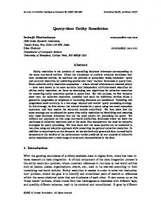
We ran our algorithm on the datasets described in Section 5.1.1. All attributes in the synthetic datasets were equally considered when assessing the quality of the clusters (the weights of all attributes are equal in Eq. 1), this amounts to eliminating the need to select the attributes that take part in the blocking key. Only the first 5 characters of every attribute value were considered (pref ix=5). We experimented on threshold values in the range [0.1, 0.55] for both the clean and dirty datasets. The results of these experiments are presented in Figure 2 and Figure 3 respectively. As can be seen in both figures 3 and 2, the PC line representing the recall when the NG constraint p = 2 (i.e, maxt∈D N G(t) ≤ 2 · minsup) was applied to the blocking, closely follows the PC line in which no NG constraint is applied. This demonstrates that the NG constraint does not harm the recall measure. On the other hand, the precision for the lower score thresholds is improved by an order of magnitude with an NG constraint of p = 2. This affect is amplified in the clean datasets (Figure 2), in which both the PC and PQ measures remain almost constant and above 0.94 for all min th values. In order to compare the results achieved by MFIBlocks to those achieved by the blocking methods surveyed in [9], we compared the average f-measure achieved by MFIBlocks when run with an SN constraint parameter p = 2 to the average f-measure achieved by the highest performing algorithm on that dataset, as reported in [9]. This comparison is detailed in Table 6. The RR measures are very high for almost all blocking methods on all dataset sizes (> 0.95) so we did detail this comparison. The actual f-measure values and standard deviations for the competing algorithms were optimistically estimated from the charts in [9]. When comparing the f-measure achieved by the MFIBlocks algorithm on the clean datasets to those achieved by the Q-gram indexing method [3] in Table 6, it can be seen that in the clean datasets results are similar for the smaller datasets, but while the effectiveness of other blocking algorithms decreases as the size of the database increases, this is not observed for the MFIBlocks algorithm. Indeed, the average f-measure for clean datasets is 0.96 with a small standard deviation regardless of the database size. According to the results on the dirty datasets, the MFIBlocks is more resilient to typographical errors and alterations in the data. Figure 4 displays the runtime of the algorithm on the datasets of various sizes. As can be seen the runtime growth is approximately linear with the database size for both the clean and dirty datasets.

5.2.2

The effects of the prefix size

type Clean Clean Clean Clean Dirty Dirty Dirty Dirty

MFIBlocks F-measure comparison to highest scoring blocking methods Algorithm Avg F-measure F-measure STDev MFIBlocks Avg F-measure Q-gram indexing 0.9 0.04 0.958 Q-gram indexing 0.9 0.04 0.965 Q-gram indexing 0.88 0.06 0.967 Q-gram indexing 0.8 0.2 0.958 Q-gram indexing 0.8 0.1 0.905 Q-gram indexing 0.79 0.12 0.888 Q-gram indexing 0.78 0.12 0.897 Q-gram indexing 0.7 0.2 0.88

size 1000 5000 10000 50000 1000 5000 10000 50000

MFIBlocks F-measure stdev 0.013 0.0085 0.001 0.001 0.07 0.061 0.05 0.1

1

1

0.9

0.9

0.8

0.8

0.8

0.7

0.7

0.7

0.7

0.6

0.6

0.6

0.6

0.5 0.4

0.5 0.4

0.3

0.3

0.2

results

1 0.9

0.8

results

1 0.9

results

results

Table 6: Comparison table for synthetic datasets

0.5

0.4

0.3

0.3

0.2

0.2

0.2

0.1

0.1

0.1

0

0

0.1

0

0

0.1

0.2

0.3

0.4

0.5

0.6

0 0

0

0.1

0.2

min threshold

0.3

0.4

0.5

0.1

PQ

F-measure

PC-NG2

F-measure-NG2

RR

PC

PQ

F-measure

PC-NG2

PQ-NG2

0.8

0.7

0.7

0.6

0.6

0.5

0.5

1

0.6

0.6

0.5

0.4 0.3

0.1

0.1

0

0

0 min thresholds F-measure

PC-NG2

0.3

0.3

0.4

0.5

0.4

(c) Clean 10000

F-measure-NG2

RR

PC

PQ

F-measure

PC-NG2

PQ-NG2

0.5

0.6

F-measure-NG2

0 0.2

0.3

0.4

0.5

0.6

0

0.1

0.2

0.3

min threshold

0.6 RR

PQ-NG2

PC-NG2

0.1

0.1

min threshold PQ-NG2

F-measure

0.2

0

0.2

PQ

0.5

0.4

0.1

PQ

0.2

PC

(b) Dirty 5000

0.7

0.2

0.1

RR

0.8

0.2

PC

0.1

F-measure-NG2

0.9

0.2

RR

0

min thresholds PQ-NG2

1

0.3

0

PC-NG2

0.7

0.3

0.6

F-measure

0.8

0.4

0.5

PQ

0.9

0.3

0.4

PC

(a) Dirty 1000

0.4

0.3

0.6

F-measure-NG2

results

1 0.9

results

results

1

0.8

0.2

0.5

min threshold

(b) Clean 5000

0.9

0.1

0.4

min thresholds PQ-NG2

(a) Clean 1000

0

0.3

results

PC

0.2

0.6 RR

RR

0.5

0.4

PC

PQ

F-measure

PC-NG2

0.4

0.5

0.6

min threshold PQ-NG2

F-measure-NG2

RR

PC

PQ

F-measure

PC-2NG

PQ-2NG

F-measure-2NG

F-measure-NG2

(c) Dirty 10000

(d) Clean 50000

(d) Dirty 50000

Figure 3: Performance on dirty datasets

Figure 2: Performance on clean datasets 800 700

5.2.3 The effects of attribute correspondences Almost all entity resolution approaches assume a correspondence between the attributes in the various sources is available, and thus reduce the problem to finding duplicates in a single table. The MFIBlocks algorithm does not perform any attribute specific indexing

600 500 seconds

We tested the effect different prefix sizes have on the outcome of the MFIBlocks algorithm. As can be seen in Figures 5 and 6, limiting the length of the attribute values considered by the algorithm had little affect on results but increased performance drastically. We ran the MFIBlocks algorithm on both the clean and dirty versions of the artificially generated database containing 5000 records. Each execution processed a different version of the database according to the configured prefix. The prefixes examined were 3, 5, 7, 10, 15, 20 and 30. In both the clean and dirty databases it can be seen that the average and maximal f-measure stay pretty much the same. On the other hand, the runtime increases linearly as the prefixes become longer. The f-measure stability can be attributed first to the fact that the prefix of an attribute value has a stronger ability to indicate similarity than the rest of the characters. This intuition is also incorporated into the Jaro-Winkler similarity metric [8] which gives more favorable ratings to strings that match from the beginning. A second cause for the f-measure stability is the fact that matching records tend to match in many attributes. Therefore, the combination of prefixes from several attributes, which are effectively discovered by the MFI mining algorithm, are a strong indicator of a match.

400 300 200 100 0 0

10000

20000

30000

40000

50000

60000

database size Clean Datasets

Dirty Datasets

Figure 4: Runtime vs. dataset size for clean and dirty datasets

or comparison and may therefore operate on a database with only a partial correspondence. We set out to investigate MFIBlocks performance on a few partial correspondence scenarios. The artificially generated datasets created by FEBRL [11] contain twelve attributes: ‘given name’, ‘surname’, ‘street number’, ‘address 1’, ‘address 2’, ‘suburb’, ‘postcode’, ‘state’, ‘date of birth’, ‘age’, ‘phone’ and ‘social security number’. Let us assume that such a generated database originated from two sources. Each source contains all the information depicted in the attributes but their distribution over the attributes may be different and of course the same attribute may have a different name in each source. For example, the attribute containing the first name may be called ‘First Name‘ in one source and ‘Given Name’ in the other. If the user is unsure

1

1

0.9

0.9

0.8

0.8 0.7

0.6

0.6 results

f-measure

0.7

0.5 0.4

0.5 0.4

0.3

0.3

0.2

0.2

0.1

0.1

0 0

5

10

15

20

25

30

0

35

0

2

4

6

prefix

Average f-measure-dirty

Max f-measure-dirty

8

10

12

14

Distinct ids Average f-measure-clean

Max f-measure-clean

Avg PC

Figure 5: F-measure vs. Prefix length

Avg PQ

Avg F-measure

Figure 7: MFIBlocks results vs. number of distinct ids 1

100 0.9 90 0.8 80 0.7 70 results

seconds

0.6 60 50

0.5 0.4

40 0.3 30 0.2 20 0.1 10 0 0

0 0

5

10

15

20

25

30

0.1

0.2

35

0.3

0.4

0.5

min threshold

prefix RR runtime-dirty

PC

PQ

F-measure

PC-NG2

PQ-NG2

F-measure-NG2

runtime-clean

Figure 8: Restaurants Dataset

Figure 6: Runtime in seconds vs. prefix length

as how to build the attribute correspondence, he may decide to assign the same ids to fields from different sources (see the algorithm setup section 4.1). For example, let us say that the first source contains the two attributes ‘given name’ and ‘surname’ but that the other source contains attributes ‘name1’ and ‘name2’. The user does not know whether to map ‘given name’ to ‘name1’ or to ‘name2’. A possible solution would be to create two fields in the integrated table ‘integrated name’ and ‘integrated surname’ which will contain ‘given name’ and ‘surname’ from the first source and ‘name1’, ‘name2’ from the second source respectively. Both fields, ‘integrated name’ and ‘integrated surname’ will be assigned the same id. In this setting, identical values from ‘name1’, ‘name2’,‘given name’ and ‘surname’ will be considered as the same item by the algorithm. We tested eight different scenarios with a different number of distinct ids. In each scenario a different group of attributes was assigned the same id (see Table 7). We ran MFIBlocks on each of these scenarios on the dirty version of the dataset containing 1000 records. The min thresholds used were in the range [0.1,0.5], and the NG constraint was set to p = 2. The average PC, PQ and f-measure for each number of distinct ids is presented in Figure 7. As expected, the precision (PQ) is highest when all correspondences are correctly mapped out, i.e, when the number of distinct ids is 12, and lowest when all the attributes were assigned the same id, confirming that the additional knowledge regarding the attribute correspondences enables more accurate clustering of the tuples. The reason for this is that two identical values representing different things such as ‘surname’ and ‘given name’, do not receive the same id and therefore do not contribute to an MFI’s score. In the PC measure there are only slight fluctuations around 0.9 which is also expected because giving the same id to non-related attributes

should not harm recall because this can only contribute to an MFI’s score. Figure 7 demonstrates that the average f-measure is more or less stable as a function of the number of distinct ids.

5.2.4

Real datasets

The results of the proposed algorithm on the real datasets summarized in Table 5 are presented below. The performance of the MFIBlocks algorithm on these datasets will be compared to the blocking algorithms surveyed in [9]. Each blocking algorithm reported in [9] was run with three different blocking keys and various parameter settings. For each dataset we will compare MFIBlocks to the highest performing algorithm on that dataset, as reported in [9].

5.2.5

Restaurants dataset

All attributes in the Restaurants dataset were equally considered when assessing the quality of the clusters (the weights of all attributes are equal in Eq. 1), this amounts to eliminating the need to select the attributes that take part in the blocking key. The results achieved for various values of the threshold parameter are provided in figure 8. We compared the results achieved by the MFIBlocks algorithm (over all NG constraints and all minimum score thresholds) to those achieved by various blocking algorithms surveyed in [9]. In particular, we compared our results to those achieved by the highest performing algorithm on the restaurants dataset, the suffix array based indexing algorithm [12]. The comparison is given in Table 8 (note, the values in the table were optimistically estimated from the charts in [9]). In the RR measure both records behave fairly the same (RR > 0.99).

5.2.6

Cora dataset

0.6

Scenario 1 2 3 4 5 6 7 8

Attributes with same id None Given Name, Surname Address1, Address2 Given Name , Surname Address1, Address2 Street number,Address1,Address2,suburb,postcode,state Given Name,Surname Street number,Address1,Address2,suburb,postcode,state Given Name,Surname Street number,Address1,Address2,suburb,postcode,state Date of birth, age phone, social security id All fields

Total number of distinct attribute ids 12 11 11 10 7 6 3 1

Table 7: Attribute correspondence scenarios Comparison to highest performing algorithm on Restaurants Alg Average F-measure STDev suffix array 0.1 0.05 MFIBlocks 0.585 0.227

1 0.9 0.8 0.7

Table 8: Comparison table for Restaurants

results

0.6 0.5 0.4 0.3 0.2 0.1

The cora dataset contains of 1295 bibliographic entries, each entry consists of 12 fields: author, volume, title, institution, venue, address, publisher, year, pages, editor, notes and month. We limited the participating attributes to those which do not contain missing values and seem more important. These are author, title, venue and year. Since the title and author fields contain many words and are relatively long, the algorithm considered only the first 30 characters of these fields. According to [9], the highest performing algorithm for this dataset was the standard blocking algorithm, the comparison is given in Table 9. The RR measure for both algorithms is similar and in both cases > 0.95. The results of MFIBlocks are displayed in Figure 9. In this dataset, the NG constraint had only little affect on the precision. The reason for this is that the clusters in the Cora dataset are relatively large when compared to its size, (it has duplicate clusters of size greater than 50). The blocks created when using a large minsup in a relatively small database create a blocking which can satisfy the NG constraint even for low thresholds. Therefore, the affect of the NG constraint in this dataset is moderate. Comparison to highest performing algorithm on Cora Alg Average F-measure STDev Standard blocking 0.55 0.05 MFIBlocks 0.713 0.07 Table 9: Comparison table for Cora

5.2.7 Census dataset All attributes in the Census dataset participate in the algorithm (their weights are > 0) although the first and last name fields were configured with a higher weight than the rest of the attributes (middle initial, zip code). The results of the MFIBlocks algorithm on this dataset are presented in Figure 10. According to [9], the highest performing algorithms for this dataset were the standard blocking and the threshold based canopy cluster-

0 0

0.1

0.2

0.3

0.4

0.5

0.6

min threshold RR

PC

PQ

F-measure

PC-NG2

PQ-NG2

F-measure-NG2

Figure 9: Cora Dataset

ing [2] algorithms, the comparison is given in Table 10. The RR measure for both algorithms is similar and in both cases > 0.95. Comparison to highest performing algorthim on Census Alg Average F-measure STDev Standard blocking 0.57 0.13 Threshold-based Canopy Clustering 0.55 0.1 MFIBlocks 0.77 0.11 Table 10: Comparison table for Census

5.2.8

Amazon-GoogleProducts dataset

The Amazon-GoogleProducts dataset originates from the e-commerce domain. It contains 4589 records and 1300 matches which were collected and annotated by the authors of [23]. Each tuple contains the product’s title, description, manufacturer and price. We compared the performance of MFIBlocks on this dataset with the results achieved by the non-learning entity resolution approaches evaluated in [23]. These include COSY, a state of the art commercial system for entity resolution, whose name cannot be disclosed, PPJoin [25] which is a match approach involving efficient similarity joins and FellegiSunter [10]. These approaches were run with an optimized threshold for the final match decision. According to [23], using only the title attribute for this matching task proved to provide higher results for all the above approaches. Therefore, we configured MFIBlocks to consider only the title attribute as well. On this task no approach received an F-measure higher than 0.62 with COSY being the top performing approach, followed by the FellegiSunter approach with an F-measure of 0.5. The maximum

1 0.9 0.8

results

0.7

[3]

0.6 0.5 0.4

[4]

0.3 0.2 0.1 0 0

0.1

0.2

0.3

0.4

0.5

0.6

[5]

min threshold RR

PC

PQ

F-measure

PC-NG4

PQ-NG4

F-measure-NG4

Figure 10: Census Dataset [6] F-measure achieved by the MFIBlocks algorithm was 0.52 as can be seen in Figure 11. It is important to note that one of the reasons MFIBlocks achieved a relatively high f-measure is the fact that it creates overlapping blocks. This isn’t the case for the algorithms evaluated in [23], which create strictly disjoint tuple sets. Overlapping blocks add a dimension of uncertainty to the final deduplicated dataset because a tuple may be assigned to more than one block. This uncertainty comes with the benefit of increased recall.

[7]

[8]

[9]

1

[10]

0.9 0.8 0.7 results

0.6 0.5

[11]

0.4 0.3 0.2 0.1 0 0

0.1

0.2

0.3

0.4

0.5

0.6

min thresholds RR

PC

PQ

F-measure

PC-NG5

PQ-NG5

F-measure-NG5

[12]

Figure 11: Amazon-GoogleProducts Dataset

6. CONCLUSIONS We presented an algorithm aimed at clustering dataset tuples in order to enable more efficient entity resolution to be carried out. The new algorithm eliminates the need to construct a complex blocking key thus making it simpler to conduct the task of blocking the dataset to be cleaned. Since the algorithm is based on mining maximal frequent itemsets, a tuple may be viewed as a sequence of items, where each item is part of an attribute value. Since the algorithm does not perform any attribute specific indexing or comparison, it performs well with only a partial correspondence between the attributes in the integrated sources. We exhibited the effectiveness and efficiency of the algorithm on both real and synthetic datasets and compared it to other known blocking methods.

7. REFERENCES [1] M. Hernandez, M. A. Hern’andez, and S. Stolfo, “Real-world data is dirty: Data cleansing and the merge/purge problem,” Data Mining and Knowledge Discovery, vol. 2, pp. 9–37, 1998. [2] A. McCallum, K. Nigam, and L. H. Ungar, “Efficient clustering of high-dimensional data sets with application to

[13]

[14]

[15]

[16]

[17]

reference matching,” in KDD ’00: Proceedings of the sixth ACM SIGKDD international conference on Knowledge discovery and data mining. New York, NY, USA: ACM, 2000, pp. 169–178. T. C. Rohan Baxter, Peter Christen, “A comparison of fast blocking methods for record linkage,” 2003. G. Grahne and J. Zhu, “Fast algorithms for frequent itemset mining using fp-trees,” IEEE TRANSACTIONS ON KNOWLEDGE AND DATA ENGINEERING, vol. 17, no. 10, pp. 1347–1362, 2005. L. Parsons, “Evaluating subspace clustering algorithms,” in in Workshop on Clustering High Dimensional Data and its Applications, SIAM International Conference on Data Mining (SDM 2004, 2004, pp. 48–56. S. Chaudhuri, V. Ganti, and R. Motwani, “Robust identification of fuzzy duplicates,” in In ICDE, 2005, pp. 865–876. F. Naumann and M. Herschel, “An introduction to duplicate detection,” Synthesis Lectures on Data Management, vol. 2, no. 1, pp. 1–87, 2010. W. E. Winkler, “Improved decision rules in the fellegi-sunter model of record linkage,” in Proceedings of the Section on Survey Research Methods, American Statistical Association, 1993, pp. 274–279. P. Christian, “A survey of indexing techniques for scalable record linkage and deduplication,” 2010. I. P. Fellegi and A. B. Sunter, “A theory for record linkage,” Journal of the American Statistical Association, vol. 64, no. 328, pp. 1183–1210, 1969. [Online]. Available: http://dx.doi.org/10.2307/2286061 P. Christen, “Febrl -: an open source data cleaning, deduplication and record linkage system with a graphical user interface,” in KDD ’08: Proceeding of the 14th ACM SIGKDD international conference on Knowledge discovery and data mining. New York, NY, USA: ACM, 2008, pp. 1065–1068. A. Aizawa and K. Oyama, “A fast linkage detection scheme for multi-source information integration,” in WIRI ’05: Proceedings of the International Workshop on Challenges in Web Information Retrieval and Integration. Washington, DC, USA: IEEE Computer Society, 2005, pp. 30–39. L. Jin, C. Li, and S. Mehrotra, “Efficient record linkage in large data sets,” in DASFAA ’03: Proceedings of the Eighth International Conference on Database Systems for Advanced Applications. Washington, DC, USA: IEEE Computer Society, 2003, p. 137. M. Bilenko, “Adaptive blocking: Learning to scale up record linkage,” in In Proceedings of the 6th IEEE International Conference on Data Mining (ICDM-2006, 2006, pp. 87–96. R. Agrawal, T. Imielinski, and A. N. Swami, “Mining association rules between sets of items in large databases,” in Proceedings of the 1993 ACM SIGMOD International Conference on Management of Data, Washington, D.C., May 26-28, 1993, P. Buneman and S. Jajodia, Eds. ACM Press, 1993, pp. 207–216. J. Han and M. Kamber, Data Mining: Concepts and Techniques (The Morgan Kaufmann Series in Data Management Systems), 1st ed. Morgan Kaufmann, September 2000. [Online]. Available: http://www.amazon.com/exec/obidos/redirect B. Goethals and M. J. Zaki, “Advances in frequent itemset mining implementations: Report on fimi’03,” in SIGKDD

Explorations, 2003, p. 2004. [18] M. Weis and F. Naumann, “Dogmatix tracks down duplicates in xml,” in SIGMOD ’05: Proceedings of the 2005 ACM SIGMOD international conference on Management of data. New York, NY, USA: ACM, 2005, pp. 431–442. [19] X. Dong, A. Halevy, and C. Yu, “Data integration with uncertainty,” in Proc. 33rd Int. Conf. on Very Large Data Bases, 2007, pp. 687–698. [20] A. Gal, M. Martinez, G. Simari, and V. Subrahmanian, “Aggregate query answering under uncertain schema mappings,” in Proc. 25th Int. Conf. on Data Engineering, 2009, pp. 940–951. [21] W. E. Winkler, “The state of record linkage and current research problems,” Statistical Research Division, U.S. Bureau of the Census, Tech. Rep., 1999. [22] G. Salton, A. Wong, and C. S. Yang, “A vector space model for automatic indexing,” Commun. ACM, vol. 18, no. 11, pp. 613–620, November 1975. [Online]. Available: http://dx.doi.org/10.1145/361219.361220 [23] H. K¨opcke, A. Thor, and E. Rahm, “Evaluation of entity resolution approaches on real-world match problems,” PVLDB, vol. 3, no. 1, pp. 484–493, 2010. [24] M. Elfeky, V. Verykios, and A. Elmagarmid, “Tailor: A record linkage toolbox,” 2002. [25] C. Xiao, W. Wang, X. Lin, and J. X. Yu, “Efficient similarity joins for near duplicate detection,” in WWW ’08: Proceeding of the 17th international conference on World Wide Web. New York, NY, USA: ACM, 2008, pp. 131–140. [Online]. Available: http://dx.doi.org/10.1145/1367497.1367516