Big-Data ER Challenges ... Algorithmic Foundations of ER. 3. Scaling ER to Big-Data ...... LDA-ER Model α. ⫠Entity l
Entity Resolution: Tutorial Entity Resolution: Tutorial Li Getoor Lise G t
Ashwin Machanavajjhala
University of Maryland College Park MD College Park, MD
Duke University Durham, NC ,
http://www.cs.umd.edu/~getoor/Tutorials/ER_VLDB2012.pdf http://goo.gl/f5eym
What is Entity Resolution? Problem of identifying and linking/grouping different manifestations of the same real world object. f f j Examples of manifestations and objects: p j • Different ways of addressing (names, email addresses, FaceBook accounts) the same person in text. • Web pages with differing descriptions of the same business. • Different photos of the same object. • …
Ironically, Entity Resolution has many duplicate names Record linkage Coreference resolution
Duplicate detection
Reference reconciliation
Fuzzy match y
Object consolidation Object consolidation Object identification
Deduplication Approximate match
Entity clustering Entity clustering
Identity uncertainty
Hardening soft databases Doubles
Merge/purge
Household matching Household matching
Householdingg
Reference matchingg
ER Motivating Examples • • • • • • • •
Linking Census Records Public Health Public Health Web search Comparison shopping Comparison shopping Counter‐terrorism Spam detection Spam detection Machine Reading …
ER and Network Analysis
before
after
Motivation: Network Science • Measuring the topology of the internet … using traceroute
IP Aliasing Problem [Willinger et al. 2009]
IP Aliasing Problem [Willinger et al. 2009]
Traditional Challenges in ER • Name/Attribute ambiguity
Thomas Cruise Thomas Cruise
Michael Jordan
Traditional Challenges in ER • Name/Attribute ambiguity Errors due to data entry • Errors due to data entry
Traditional Challenges in ER • Name/Attribute ambiguity Errors due to data entry • Errors due to data entry • Missing Values
[Gill et al; Univ of Oxford 2003]
Traditional Challenges in ER • • • •
Name/Attribute ambiguity Errors due to data entry Errors due to data entry Missing Values Changing Attributes Changing Attributes
• Data formatting
• Abbreviations / Data Truncation /
Big‐Data ER Challenges
Big‐Data ER Challenges • Larger and more Datasets – Need efficient parallel techniques
• More Heterogeneity M H t it – Unstructured, Unclean and Incomplete data. Diverse data types. – No longer just matching names with names, but Amazon profiles with No longer just matching names with names, but Amazon profiles with browsing history on Google and friends network in Facebook.
Big‐Data ER Challenges • Larger and more Datasets – Need efficient parallel techniques
• More Heterogeneity M H t it – Unstructured, Unclean and Incomplete data. Diverse data types.
• More linked More linked – Need to infer relationships in addition to “equality”
• Multi‐Relational – Deal with structure of entities (Are Walmart and Walmart Pharmacy the same?)
• Multi‐domain l d – Customizable methods that span across domains
• Multiple applications Multiple applications (web search versus comparison shopping) (web search versus comparison shopping) – Serve diverse application with different accuracy requirements
Outline 1. 2 2. 3. 4 4.
Abstract Problem Statement Algorithmic Foundations of ER Algorithmic Foundations of ER Scaling ER to Big‐Data Challenges & Future Directions Challenges & Future Directions
Outline 1. Abstract Problem Statement 2 Algorithmic Foundations of ER 2. Algorithmic Foundations of ER a) b) c) d)
Data Preparation and Match Features Pairwise ER Constraints in ER Algorithms • • •
Record Linkage Record Linkage Deduplication Collective ER
3. Scaling ER to Big‐Data 4. Challenges & Future Directions
5 minute break
Outline 1. Abstract Problem Statement 2 Algorithmic Foundations of ER 2. Algorithmic Foundations of ER 3. Scaling ER to Big‐Data a) Blocking/Canopy Generation Blocking/Canopy Generation b) Distributed ER
4. Challenges & Future Directions Challenges & Future Directions
Outline 1. 2 2. 3. 4 4.
Abstract Problem Statement Algorithmic Foundations of ER Algorithmic Foundations of ER Scaling ER to Big‐Data Challenges & Future Directions Challenges & Future Directions
Scope of the Tutorial • What we cover: – Fundamental algorithmic concepts in ER – Scaling ER to big datasets – Taxonomy of current ER algorithms
• What we do not cover: – – – – – –
Schema/ontology resolution Schema/ontology resolution Data fusion/integration/exchange/cleaning Entity/Information Extraction Privacy aspects of Entity Resolution Details on similarity measures Technical details and proofs Technical details and proofs
ER References • Book / Survey Articles – Data Quality and Record Linkage Techniques [T Herzog F Scheuren W Winkler Springer ’07] [T. Herzog, F. Scheuren, W. Winkler, Springer, 07] – Duplicate Record Detection [A. Elmagrid, P. Ipeirotis, V. Verykios, TKDE ‘07] – An Introduction to Duplicate Detection [F. Naumann, M. Herschel, M&P y ] synthesis lectures 2010] – Evaluation of Entity Resolution Approached on Real‐world Match Problems [H. Kopke, A. Thor, E. Rahm, PVLDB 2010] – Data Matching [P. Christen, Springer 2012]
• Tutorials – Record Linkage: Similarity measures and Algorithms [N. Koudas, S. Sarawagi, D. Srivatsava SIGMOD ‘06] – Data fusion‐‐Resolving data conflicts for integration [X. Dong, F. Naumann VLDB ‘09] – Entity Resolution: Theory, Practice and Open Challenges Entity Resolution: Theory Practice and Open Challenges http://goo.gl/Ui38o [L. Getoor, A. Machanavajjhala AAAI ‘12]
PART 1 PART 1 ABSTRACT PROBLEM STATEMENT ABSTRACT PROBLEM STATEMENT
Abstract Problem Statement Real World
Digital World
Records / / Mentions
Deduplication Problem Statement • Cluster the records/mentions that correspond to same entity y
Deduplication Problem Statement • Cluster the records/mentions that correspond to same entity y – Intensional Variant: Compute cluster representative
Record Linkage Problem Statement • Link records that match across databases A
B
Reference Matching Problem • Match noisy records to clean records in a reference table
Reference Table bl
Abstract Problem Statement Real World
Digital World
Deduplication Problem Statement
Deduplication with Canonicalization
Graph Alignment (& motif search) Graph 1
Graph 2
Relationships are crucial
Relationships are crucial
Notation • • • • • •
R: set of records / mentions (typed) H: set of relations / hyperedges (typed) H: set of relations / hyperedges M: set of matches (record pairs that correspond to same entity ) N: set of non matches (record pairs corresponding to different entities) N: set of non‐matches ( d i di t diff t titi ) E: set of entities L set of links L: set of links
• TTrue (M (Mtrue, N Ntrue, EEtrue, LLtrue): according to real world ) di l ld vs Predicted (Mpred, Npred, Epred, Lpred ): by algorithm
Relationship between Mtrue and Mpred • Mtrue (SameAs , Equivalence) (Similar representations and similar attributes) • Mpred (Similar representations and similar attributes) Mtrue
RxR
Mpred
Metrics • Pairwise metrics – Precision/Recall, F1 – # of predicted matching pairs
• Cluster level metrics – purity, completeness, complexity – Precision/Recall/F1: Cluster‐level, closest cluster, MUC, B Precision/Recall/F1: Cluster level closest cluster MUC B3 , Rand Index – Generalized merge distance [Menestrina et al, PVLDB10]
• Little work that evaluations correct prediction of links
Typical Assumptions Made • Each record/mention is associated with a single real world entity. y
• In record linkage, no duplicates in the same source • If two records/mentions are identical, then they are true If two records/mentions are identical then they are true matches
( ( , ) ε ) Mtrue
ER versus Classification Finding matches vs non‐matches is a classification problem • Imbalanced: typically O(R) matches, O(R^2) non‐matches • Instances are pairs of records. Pairs are not IID
( , ) ε Mtrue AND
( , ) ε Mtrue ( , ) ε
( ( , ) ε ) ε Mtrue
ER vs (Multi‐relational) Clustering Computing entities from records is a clustering problem • In typical clustering algorithms (k‐means, LDA, etc.) number of clusters is a constant or sub linear in R. number of clusters is a constant or sub linear in R. • In In ER: number of clusters is linear in R, and average ER: number of clusters is linear in R and average cluster size is a constant. Significant fraction of clusters are singletons. g
PART 2 PART 2 ALGORITHMIC FOUNDATIONS OF ER ALGORITHMIC FOUNDATIONS OF ER
Outline of Part 2 a) Data Preparation and Match Features b) Pairwise ER –
Determining whether or not a pair of records match
c) Constraints in ER 5 minute break
d) Algorithms – – –
Record linkage (Propagation through exclusitivity negative constraint), Deduplication (Propagation through transitivity positive constraint), Collective (Propagation through General Constraints)
MOTIVATING EXAMPLE: MOTIVATING EXAMPLE: BIBLIOGRAPHIC DOMAIN
Entities & Relations in Bibliographic Domain Wrote
Paper p Title # of Authors Topic Word1 Word 2 … WordN Cites
Author
Name Research Area
WorksAt
I tit ti Institution Name
Author Mention NameString
Institute Mention NameString
Paper Mention TitleString
AppearsIn pp
Venue
: entity relationships : co‐occurrence relationships : resolution relationships
Name
Venue Mention NameString g
PART 2 PART 2‐a DATA PREPARATION & DATA PREPARATION & MATCH FEATURES
Normalization •
Schema normalization – Schema Matching – e.g., contact number and phone number – Compound attributes – C d tt ib t f ll dd full address vs str,city,state,zip t it t t i – Nested attributes • List of features in one dataset (air conditioning, parking) vs each feature a boolean attribute – Set valued attributes • Set of phones vs primary/secondary phone – Record segmentation from text Record segmentation from text
•
Data normalization – Often convert to all lower/all upper; remove whitespace – detecting and correcting values that contain known typographical errors or d i d i l h i k hi l variations, – expanding abbreviations and replacing them with standard forms; replacing nicknames with their proper name forms nicknames with their proper name forms – Usually done based on dictionaries (e.g., commercial dictionaries, postal addresses, etc.)
Matching Features • For two references x and y, compute a “comparison” vector of similarity scores of component attribute. – [ 1st‐author‐match‐score, paper‐match‐score, venue‐match‐score, year‐match‐score, …. ]
• Similarity scores y – Boolean (match or not‐match) – Real values based on distance functions
Summary of Matching Features Handle H dl Typographical errors
• •
Equality on a boolean predicate Edit distance – Levenstein, Smith‐Waterman, Affine
•
•
• Vector Based – Cosine Cosine similarity, TFIDF similarity, TFIDF Good for Text like reviews/ tweets
Alignment‐based or Two‐tiered – Jaro‐Winkler, Soft‐TFIDF, Monge‐Elkan
•
Phonetic Similarity – Soundex
Set similarity – Jaccard, Dice
•
Good for Names
• • •
Translation‐based Numeric distance between values Domain‐specific p
Useful packages Useful packages: – SecondString, http://secondstring.sourceforge.net/ – Simmetrics: http://sourceforge.net/projects/simmetrics/ – LingPipe, http://alias‐i.com/lingpipe/index.html Li Pi htt // li i /li i /i d ht l
Useful for abbreviations, alternate names. alternate names.
Relational Matching Features • Relational features are often set‐based – Set of coauthors for a paper – Set of cities in a country f ii i – Set of products manufactured by manufacturer
• Can use set similarity functions mentioned earlier – Common Neighbors: Intersection size – Jaccard Jaccard’ss Coefficient: Normalize by union size Coefficient: Normalize by union size – Adar Coefficient: Weighted set similarity
• Can reason about similarity in sets of values C b t i il it i t f l – Average or Max – Other aggregates
PART 2 b PART 2‐b PAIRWISE MATCHING
Pairwise Match Score Problem: Given a vector of component‐wise similarities for a pair of records (x,y), compute P(x and y match). Solutions: 1. Weighted sum or average of component‐wise similarity scores. Threshold determines match or non‐match. –
0.5*1st‐author‐match‐score + 0.2*venue‐match‐score + 0.3*ppaper‐match‐score p .
–
Hard to pick weights. • •
–
Match on last name match more predictive than login name. Match on “Smith” Match on Smith less predictive than match on less predictive than match on “Getoor” Getoor or or “Machanavajjhala”.
Hard to tune a threshold.
Pairwise Match Score Problem: Given a vector of component‐wise similarities for a pair of records (x,y), compute P(x and y match). Solutions: 1. Weighted sum or average of component‐wise similarity scores. Threshold determines match or non‐match. 2 Formulate rules about what constitutes a match. 2. Formulate rules about what constitutes a match –
(1st‐author‐match‐score > 0.7 AND venue‐match‐score > 0.8) OR (paper‐match‐score > 0.9 AND venue‐match‐score > 0.9)
–
M Manually formulating the right set of rules is hard. ll f l ti th i ht t f l i h d
Basic ML Approach • r = (x,y) is record pair, is comparison vector, M matches, U non‐ matches • Decision rule
P( | r M ) R P( | r U )
R t r Match R t r Non - Match
Fellegi & Sunter Model [FS, Science ‘69] • r = (x,y) is record pair, is comparison vector, M matches, U non‐ matches • Decision rule
P( | r M ) R P( | r U )
R tl r Match tl R tu r Potential Match R tu r Non - Match • Naïve Bayes Assumption: P( | r M ) i P( i | r M )
ML Pairwise Approaches • Supervised machine learning algorithms – Decision trees • [Cochinwala [Co hin ala et al, IS01] et al IS01]
– Support vector machines • [Bilenko & Mooney, KDD03]; [Christen, KDD08]
– Ensembles of classifiers Ensembles of classifiers • [Chen et al., SIGMOD09]
– Conditional Random Fields (CRF) • [Gupta & Sarawagi, VLDB09] [Gupta & Sarawagi VLDB09]
• Issues: – Training Training set generation set generation – Imbalanced classes – many more negatives than positives (even after eliminating obvious non‐matches … using Blocking) – Misclassification cost Misclassification cost
Creating a Training Set is a key issue • Constructing a training set is hard – since most pairs of records are “easy non‐matches”. y – 100 records from 100 cities. – Only 106 pairs out of total 108 (1%) come from the same city
• Some pairs are hard to judge even by humans – Inherently ambiguous • E.g., Paris Hilton (person or business)
– Missing attributes • Starbucks, Toronto vs Starbucks, Queen Street ,Toronto
Avoiding Training Set Generation • Unsupervised / Semi‐supervised Techniques – EM based techniques to learn parameters • [Winkler ‘06, Herzog et al ’07]
– Generative Models • [Ravikumar & Cohen, UAI04] & Cohen UAI04]
• Active Learning – Committee of Classifiers • [Sarawagi et al KDD ’00, Tajeda et al IS ‘01]
– Provably optimizing precision/recall Provably optimizing precision/recall • [Arasu et al SIGMOD ‘10, Bellare et al KDD ‘12]
– Crowdsourcing • [Wang et al VLDB ‘12, Marcus et al VLDB ’12, …] [W t l VLDB ‘12 M t l VLDB ’12 ]
Committee of Classifiers [Tejada et al, IS ‘01]
Active Learning with Provable Guarantees • Most active learning techniques minimize 0‐1 loss [Beygelzimer et al NIPS 2010].
• However, ER is very imbalanced: – Number of non‐matches > 100 * number of matches. – Classifying all pairs as “non‐matches” has low 0‐1 loss ( Transitivity • Often pairwise ER algorithm output “inconsistent” results – (x, y) ε Mpred , (y,z) ε Mpred , but (x,z) ε Mpred
• Idea: Correct this by adding additional matches using transitive closure l • In certain cases, this is a bad idea. In certain cases this is a bad idea – Graphs resulting from pairwise ER have diameter > 20 [Rastogi et al Corr et al Corr ‘12] 12]
Added by Transitive Transitive Closure
• Need clustering solutions that deal with this problem directly by reasoning about records jointly.
Clustering‐based ER • Resolution decisions are not made independently for each pair of records • Based on variety of clustering algorithms, but – Number of clusters unknown aprioiri – Many, many small (possibly singleton) clusters
• Often take a pair‐wise similarity graph as input • May require the construction of a cluster representative or canonical entity
Clustering Methods for ER • Hierarchical Clustering – [[Bilenko et al, ICDM 05] , ]
• Nearest Neighbor based methods – [Chaudhuri et al, ICDE 05]
• Correlation Clustering – [Soon et al CL’01, Bansal et al ML’04, Ng et al ACL’02, Ailon et al JACM’08, Elsner et al ACL’08, Elsner et al ILP‐NLP’09]
Integer Linear Programming view of ER • rxy ε {0,1}, rxy = 1 if records x and y are in the same cluster. • w+xy ε [0,1], cost of clustering x and y together [ ] g y g • w –xy ε [0,1], cost of placing x and y in different clusters
Transitive closure
Correlation Clustering
• Cluster mentions such that total cost is minimized total cost is minimi ed Solid edges contribute w+
to the objective Dashed edges contribute w –xyy to the objective xy
4
2 1 3
5
• Cost based on pairwise similarities – Additive: w+xy = pxy and w –xy = (1‐pxy) oga t c +xy = log(p og(pxy)) and w a d –xy = log(1‐p og( pxy) – Logarithmic: w
Correlation Clustering • Solving the ILP is NP‐hard [Ailon et al 2008 JACM] • A number of heuristics [Elsner et al 2009 ILP‐NLP] – Greedy BEST/FIRST/VOTE algorithms Greedy BEST/FIRST/VOTE algorithms – Greedy PIVOT algorithm (5‐approximation) – Local Search
Greedy Algorithms SStep 1: Permute the nodes according a random π 1 P h d di d Step 2: Assign record x to the cluster that maximizes Quality Start a new cluster if Quality < 0 Start a new cluster if Quality 0 – [Soon et al 2001 CL] [Soon et al 2001 CL]
• VOTE: Assign to cluster that minimizes objective function. – [Elsner et al 08 ACL] Practical Note: • Run the algorithm for many random permutations , and pick the clustering with best objective value (better than average run)
Greedy with approximation guarantees PIVOT Algorithm [Ailon et al 2008 JACM] • Pick a random (pivot) record p. (p ) p • New cluster = 2
• • •
π = {1,2,3,4} C = {{1,2,3,4}} π = {2,4,1,3} C = {{1,2}, {4}, {3}} { , , , } {{ , }, { }, { }} π = {3,2,4,1} C = {{1,3}, {2}, {4}}
When weights are 0/1, For w+xy + w–xy = 1,
1 3 4
E(cost(greedy))