Scaling Entity Resolution to Large, Heterogeneous Data with ...
Recommend Documents
a comparison may be prohibitive for big data sets if all tuple pairs are compared and hence .... tion of a blocking key in order to index or sort the database tuples.
Sep 15, 2015 - Conference on Big Data (IEEE BigData 2015), Oct 2015, Santa Clara, CA,, ... we focus on entity resolution in the Web of data, i.e., identifying.
(HHIS) through a novel framework that consists of two orthogonal layers: the ... Index TermsâInformation Integration, Entity Resolution, Blocking Methods.
Dec 1, 2016 - the blocking graph implicitly, while the entity-based strategy is independent of the blocking ..... Symbol. Entity collection. E. Duplicate entities in E. D(E) ...... linkage system: http: //datamining.anu.edu.au/linkage.html, in: PAKDD
Aug 9, 2012 - transfer learning, multi-task learning, convex optimization ... cannot be outsourced. ... source ER problem for the movies vertical in a major Internet search ... engine, we demonstrate both on a large real-world movie entity.
Dec 2, 2015 - interpretation strategies to alternative state-of-the-art ap- proaches that do not ... [31] or the Facebook Entities Graph [32]. Even though the.
function call. Note that each of these functions only operates on the key of key-value pairs and does not take the values into account. Keys can have any arbitrary ...
given different names) in many computer science domains. Examples include ... sus example, if we are able to determine that the two Jason Does refer to the ..... are available for references, this approach can be generalized to obtain better.
plications they must still be manually verified by an analyst or data curator. ... We explore different techniques for solving the collective entity resolution problem.
to simply return records that match the query name, 'S. Russell' or 'Jon Doe' exactly. In order to retrieve all the ..... entity resolution problem has received a lot of attention. We review ..... Also, none of them are actually going ...... setting,
Big-Data ER Challenges ... Algorithmic Foundations of ER. 3. Scaling ER to Big-Data ...... LDA-ER Model α. ⫠Entity l
the large and very large data sets, such as Web Data, data blocking ...... ing, they associate every entity with multiple blocks, based on the bi-/q-grams3 that are ...
over large, highly heterogeneous Information Spaces. Von der Fakultät .... the large and very large data sets, such as Web Data, data blocking techniques are typically ...... as R-Trees, similar BKs can be efficiently grouped into clusters. A new ..
tegrating information from multiple heterogeneous data sources, and making this .... Redundant Arrays of Inexpensive Disks (RAID) and Storage Area Network (SAN) ... of small files, and backup and recovery of such a file system can be ...
Data Mining and Knowledge Discovery, Volume 5, Number 3, 2001. Scaling ... the solution of a system of linear equations the size of the training data set.
three problems when one tries to scale up these systems to large data ...... and K.-R. Müller, (Eds.), Advances in Neural Information Processing Systems,. 12.
M. Bramer e-mail: [email protected]. P. Rausch et al. (eds.), Business Intelligence and Performance Management,. Advanced Information and Knowledge ...
Progressive. ER aims to efficiently resolve large datasets when limited time ...... 4.2Mâ3.7M. 37kâ11k. 1.5M anymore and is thus discarded. Complexity Analysis. .... On the other hand, for datasets with a high token overlap of matching profiles .
German Wikipedia as reference for named enti- ties. ... For many organizations there exist a number ... ple, Peter Müller the prime minister may not be mentioned.
named âHarold Knopf Merriweatherâ, and only later encounter additional information indicating there are two different people with this name (unlikely as that may ...
Named Entity Resolution Using Automatically Extracted Semantic Information. Anja Pilz and Gerhard PaaÃ. Fraunhofer Institute Intelligent Analysis and ...
data mining on a database that has been normalized using ... companies, high-profile people, etc. ... person publishes multiple articles or when a company is.
edu/linqs/ddupe), a visual analytic tool, which supports relational entity ... H. Kang is with the Institute for Advanced Computer Studies, University of Maryland ...
El Segundo, CA 90245 [email protected]. ABSTRACT. We have encountered several practical issues in performing data mining on a database that has been ...
Scaling Entity Resolution to Large, Heterogeneous Data with ...
ABSTRACT. Entity Resolution constitutes a quadratic task that typically scales to large entity collections through blocking. The resulting blocks.
Scaling Entity Resolution to Large, Heterogeneous Data with Enhanced Meta-blocking George Papadakis$ , George Papastefanatos# , Themis Palpanas^ , Manolis Koubarakis$ Paris Descartes University, France [email protected] IMIS, Research Center “Athena”, Greece [email protected] $ Dep. of Informatics & Telecommunications, Uni. Athens, Greece {gpapadis, koubarak}@di.uoa.gr ^
#
ABSTRACT Entity Resolution constitutes a quadratic task that typically scales to large entity collections through blocking. The resulting blocks can be restructured by Meta-blocking in order to significantly increase precision at a limited cost in recall. Yet, its processing can be time-consuming, while its precision remains poor for configurations with high recall. In this work, we propose new meta-blocking methods that improve precision by up to an order of magnitude at a negligible cost to recall. We also introduce two efficiency techniques that, when combined, reduce the overhead time of Metablocking by more than an order of magnitude. We evaluate our approaches through an extensive experimental study over 6 realworld, heterogeneous datasets. The outcomes indicate that our new algorithms outperform all meta-blocking techniques as well as the state-of-the-art methods for block processing in all respects.
1.
INTRODUCTION
A common task in the context of Web Data is Entity Resolution (ER), i.e., the identification of different entity profiles that pertain to the same real-world object. ER suffers from low efficiency, due to its inherently quadratic complexity: every entity profile has to be compared with all others. This problem is accentuated by the continuously increasing volume of heterogeneous Web Data; LODStats1 recorded around 1 billion triples for Linked Open Data in December, 2011, which had grown to 85 billion by September, 2015. Typically, ER scales to these volumes of data through blocking [4]. The goal of blocking is to boost precision and time efficiency at a controllable cost in recall [4, 5, 21]. To this end, it groups similar profiles into clusters (called blocks) so that it suffices to compare the profiles within each block [7, 8]. Blocking methods for Web Data are confronted with high levels of noise, not only in attribute values, but also in attribute names. In fact, they involve an unprecedented schema heterogeneity: Google Base2 alone encompasses 100,000 distinct schemata that correspond to 10,000 entity types [17]. Most blocking methods deal with these high levels of 1 2
http://stats.lod2.eu http://www.google.com/base
c 2016, Copyright is with the authors. Published in Proc. 19th Inter national Conference on Extending Database Technology (EDBT), March 15-18, 2016 - Bordeaux, France: ISBN 978-3-89318-070-7, on OpenProceedings.org. Distribution of this paper is permitted under the terms of the Creative Commons license CC-by-nc-nd 4.0
p1 p3
p5
FullName : Jack Lloyd Miller job : autoseller full name : Jack Miller Work : car vendor ‐ seller Full name : James Jordan job : car seller
p2 p4
p6
name : Erick Green profession : vehicle vendor Erick Lloyd Green car trader name : Nick Papas profession : car dealer
(a) b1 (Jack) p1 p3
b2 (Miller) p1 p3
b3 (Erick) p2 p4
b4 (Green) p2 p4
b5 (vendor) p2 p3
b6 (seller) p3 p5
b7 (Lloyd) p1 p4
p3 p4 p5 p6
b8 (car)
(b)
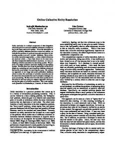
Figure 1: (a) A set of entity profiles, and (b) the corresponding blocks produced by Token Blocking. schema heterogeneity through a schema-agnostic functionality that completely disregards schema information and semantics [5]. They also rely on redundancy, placing every entity profile into multiple blocks so as to reduce the likelihood of missed matches [4, 22]. The simplest method of this type is Token Blocking [21]. In essence, it splits the attribute values of every entity profile into tokens based on whitespace; then, it creates a separate block for every token that appears in at least two profiles. To illustrate its functionality, consider the entity profiles in Figure 1(a), where p1 and p2 match with p3 and p4 , respectively; Token Blocking clusters them in the blocks of Figure 1(b). Despite the schema heterogeneity and the noisy values, both pairs of duplicates co-occur in at least one block. Yet, the total cost is 13 comparisons, which is rather high, given that the brute-force approach executes 15 comparisons. This is a general trait of redundancy-based blocking methods: in their effort to achieve high recall in the context of noisy and heterogeneous data, they produce a large number of unnecessary comparisons. These come in two forms [22, 23]: the redundant ones repeatedly compare the same entity profiles across different blocks, while the superfluous ones compare non-matching profiles. In our example, b2 and b4 contain one redundant comparison each, which are repeated in b1 and b3 , respectively; all other blocks entail superfluous comparisons between non-matching entity profiles, except for the redundant comparison p3 -p5 in b8 (it is repeated in b6 ). In total, the blocks of Figure 1(b) involve 3 redundant and 8 superfluous out of the 13 comparisons. Block Processing. To improve the quality of redundancy-based blocks, methods such as Meta-blocking [5, 7, 22], Comparison Propagation [21] and Iterative Blocking [27] aim to process them in the optimal way (see Section 2 for more details). Among these methods, Meta-blocking achieves the best balance between preci-
v1
1/6 1/7
1/8
v3
v5
v1
v2
2/5
2/6
2/5
v2
v4
v3
v4
1/5 1/4
1/5
1/2 (a)
v6
v5
v6 (b)
b'1 p1 p3
b'2 p2 p4
b'3 p3 p5
b'4 p4 p6
b'5 p5 p6 (c)
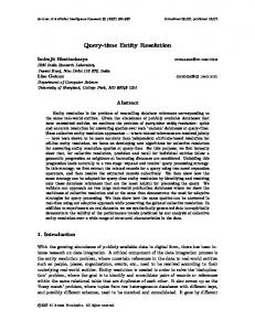
Figure 2: (a) A blocking graph extracted from the blocks in Figure 1(b), (b) one of the possible edge-centric pruned blocking graphs, and (c) the new blocks derived from it. sion and recall [22, 23], and is the focus of this work. Meta-blocking restructures a block collection B into a new one B0 that contains a significantly lower number of unnecessary comparisons, while detecting almost the same number of duplicates. It operates in two steps [7, 22, 23]: first, it transforms B into the blocking graph G B , which contains a vertex vi for every entity profile pi in B, and an edge ei, j for every pair of co-occurring profiles pi and p j (i.e., entity profiles sharing at least one block). Figure 2(a) depicts the graph for the blocks in Figure 1(b). As no parallel edges are constructed, every pair of entities is compared at most once, thus eliminating all redundant comparisons. Second, it annotates every edge with a weight analogous to the likelihood that the incident entities are matching. For instance, the edges in Figure 2(a) are weighted with the Jaccard similarity of the lists of blocks associated with their incident entity profiles. The lower the weight of an edge, the more likely it is to connect non-matching entities. Therefore, Meta-blocking discards most superfluous comparisons by pruning the edges with low weights. A possible approach is to discard all edges with a weight lower than the overall mean weight (1/4). This yields the pruned graph in Figure 2(b). The restructured block collection B0 is formed by creating a new block for every retained edge – as depicted in Figure 2(c). Note that B0 maintains the original recall, while reducing the comparisons from 13 to just 5. Open issues. Despite the significant enhancements in efficiency, Meta-blocking suffers from two drawbacks: (i) There is plenty of room for raising its precision, especially for the configurations that are more robust to recall. The reason is that they retain a considerable portion of redundant and superfluous comparisons. This is illustrated in our example, where the restructured blocks of Figure 2(c) contain 3 superfluous comparisons in b03 , b04 and b05 . (ii) The processing of voluminous datasets involves a significant overhead. The corresponding blocking graphs comprise millions of nodes that are strongly connected with billions of edges. Inevitably, the pruning of such graphs is very time-consuming; for example, a graph with 3.3 million nodes and 35.8 billion edges requires 16 hours, on average, on commodity hardware (see Section 6.3). Proposed Solution. In this paper, we describe novel techniques for overcoming both weaknesses identified above. First, we speed up Meta-blocking in two ways: (i) We introduce Block Filtering, which intelligently removes profiles from blocks, in which their presence is unnecessary. This acts as a pre-processing technique that shrinks the blocking graph, discarding more than half of its unnecessary edges, on average. As a result, the running time is also reduced to half, on average. (ii) We accelerate the creation and the pruning of the blocking graph by minimizing the computational cost for edge weighting, which is the bottleneck of Meta-blocking. Our approach reduces its running time by 30% to 70%.
In combination, these two techniques restrict drastically the overhead of Meta-blocking even on commodity hardware. For example, the blocking graph mentioned earlier is now processed within just 3 hours, instead of 16. Second, we enhance the precision of Meta-blocking in two ways: (i) We redefine two pruning algorithms so that they produce restructured blocks with no redundant comparisons. On average, they save 30% more comparisons for the same recall. (ii) We introduce two new pruning algorithms that rely on a generic property of the blocking graph: the reciprocal links. That is, our algorithms retain only the edges that are important for both incident profiles. Their recall is slightly lower than the existing techniques, but precision raises by up to an order of magnitude. We analytically examine the performance of our methods using 6 real-world established benchmarks, which range from few thousands to several million entities. Our experimental results designate that our algorithms consistently exhibit the best balance between recall, precision and run-time for the main types of ER applications among all meta-blocking techniques. They also outperform the best relevant methods in the literature to a significant extent. Contributions & Paper Organization. In summary, we make the following contributions: • We improve the running time of Meta-blocking by an order of magnitude in two complementary ways: by cleaning the blocking graph from most of its noisy edges, and by accelerating the estimation of edge weights. • We present four new pruning algorithms that raise precision by 30% to 100% at a small (if any) cost in recall. • We experimentally verify the superior performance of our new methods through an extensive study over 6 datasets with different characteristics. In this way, our experimental results provide insights into the best configuration for Meta-blocking, depending on the data and the application at hand. The code and the data of our experiments are publicly available for any interested researcher.3 The rest of the paper is structured as follows: Section 2 delves into the most relevant works in the literature, while Section 3 elaborates on the main notions of Meta-blocking. In Section 4, we introduce two methods for minimizing its running time, and in Section 5, we present new pruning algorithms that boost the precision of Meta-blocking at no or limited cost in recall. Section 6 presents our thorough experimental evaluation, while Section 7 concludes the paper along with directions for future work.
2.
RELATED WORK
Entity Resolution has been the focus of numerous works that aim to tame its quadratic complexity and scale it to large volumes of data [4, 8]. Blocking is the most popular among the proposed approximate techniques [5, 7]. Some blocking methods produce disjoint blocks, such as Standard Blocking [9]. Their majority, though, yields overlapping blocks with redundant comparisons in an effort to achieve high recall in the context of noisy and heterogeneous data [4]. Depending on the interpretation of redundancy, blocking methods are distinguished into three categories [22]: (i) The redundancy-positive methods ensure that the more blocks two entity profiles share, the more likely they are to be matching. In this category fall the Suffix Arrays [1], Q-grams Blocking [12], Attribute Clustering [21] and Token Blocking [21]. (ii) The redundancy-negative methods ensure that the most similar entity profiles share just one block. In Canopy Clustering [19], for instance, the entity profiles that are highly similar to the cur3 See http://sourceforge.net/projects/erframework for both the code and the datasets.
rent seed are removed from the pool of candidate matches and are exclusively placed in its block. (iii) The redundancy-neutral methods yield overlapping blocks, but the number of common blocks between two profiles is irrelevant to their likelihood of matching. As such, consider the single-pass Sorted Neighborhood [13]: all pairs of profiles co-occur in the same number of blocks, which is equal to the size of the sliding window. Another line of research focuses on developing techniques that optimize the processing of an existing block collection, called block processing methods. In this category falls Meta-blocking [7], which operates exclusively on top of redundancy-positive blocking methods [20, 21]. Its pruning can be either unsupervised [22] or supervised [23]. The latter achieves higher accuracy than the former, due to the composite pruning rules that are learned by a classifier trained over a set of labelled edges. In practice, though, its utility is limited, as there is no effective and efficient way for extracting the required training set from the input blocks. For this reason, we exclusively consider unsupervised Meta-blocking in this work. Other prominent block processing methods are the following: (i) Block Purging [21] aims for discarding oversized blocks that are dominated by redundant and superfluous comparisons. It automatically sets an upper limit on the comparisons that can be contained in a valid block and purges those blocks that exceed it. Its functionality is coarser and, thus, less accurate than Meta-blocking, because it targets entire blocks instead of individual comparisons. However, it is complementary to Meta-blocking and is frequently used as a pre-processing step [22, 23]. (ii) Comparison Propagation [21] discards all redundant comparisons from a block collection without any impact on recall. In a small scale, this can be accomplished directly, using a central data structure H that hashes all executed comparisons; then, a comparison is executed only if it is not contained in H. Yet, in the scale of billions of comparisons, Comparison Propagation can only be accomplished indirectly: the input blocks are enumerated according to their processing order and the Entity Index is built. This is an inverted index that points from entity ids to block ids. Then, a comparison pi -p j in block bk is executed (i.e., non-redundant) only if it satisfies the Least Common Block Index condition (LeCoBI for short). That is, if the id k of the current block bk equals the least common block id of the profiles pi and p j . Comparison Propagation is competitive to Meta-blocking, but targets only redundant comparisons. We compare their performance in Section 6.4. (ii) Iterative Blocking [27] propagates all identified duplicates to the subsequently processed blocks so as to save repeated comparisons and to detect more duplicates. Hence, it improves both precision and recall. It is competitive to Meta-blocking, too, but it targets exclusively redundant comparisons between matching profiles. We employ it as our second baseline method in Section 6.4.
3.
PRELIMINARIES
Entity Resolution. An entity profile, p, is defined as a uniquely identified collection of name-value pairs that describe a real-world object. A set of profiles is called entity collection, E. Given E, the goal of ER is to identify all profiles that describe the same realworld object; two such profiles, pi and p j , are called duplicates (pi ≡p j ) and their comparison is called matching. The set of all duplicates in the input entity collection E is denoted by D(E), with |D(E)| symbolizing its size (i.e., the number of existing duplicates). Depending on the input entity collection(s), we identify two ER tasks [4, 21, 22]: (i) Dirty ER takes as input a single entity collection with duplicates and produces as output a set of equivalence clusters. (ii) Clean-Clean ER receives two duplicate-free, but overlapping entity collections, E1 and E2 , and identifies the matching
entity profiles between them. In the context of Databases, the former task is called Deduplication and the latter Record Linkage [4]. Blocking improves the run-time of both ER tasks by grouping similar entity profiles into blocks so that comparisons are limited between co-occurring profiles. Placing an entity profile into a block is called block assignment. Two profiles, pi and p j , assigned to the same block are called co-occurring and their comparison is denoted by ci, j . An individual block is symbolized by b, with |b| denoting its size (i.e., number of profiles) and ||b|| denoting its cardinality (i.e., number of comparisons). A set of blocks B is called block collection, with |B| denoting its size (i.e., number of blocks) Pand ||B|| its cardinality (i.e., total number of comparisons): ||B|| = b∈B ||b||. Performance Measures. To assess the effectiveness of a blocking method, we follow the best practice in the literature, which treats entity matching as an orthogonal task [4, 5, 7]. We assume that two duplicate profiles can be detected using any of the available matching methods as long as they co-occur in at least one block. D(B) stands for the set of co-occurring duplicate profiles and |D(B)| for its size (i.e., the number of detected duplicates). In this context, the following measures are typically used for estimating the effectiveness of a block collection B that is extracted from the input entity collection E [4, 5, 22]: (i) Pairs Quality (PQ) corresponds to precision, assessing the portion of comparisons that involve a non-redundant pair of duplicates. In other words, it considers as true positives the matching comparisons and as false positives the superfluous and the redundant ones (given that some of the redundant comparisons involve duplicate profiles, PQ offers a pessimistic estimation of precision). More formally, PQ = |D(B)|/||B||. PQ takes values in the interval [0, 1], with higher values indicating higher precision for B. (ii) Pairs Completeness (PC) corresponds to recall, assessing the portion of existing duplicates that can be detected in B. More formally, PC = |D(B)|/|D(E)|. PC is defined in the interval [0, 1], with higher values indicating higher recall. The goal of blocking is to maximize both PC and PQ so that the overall effectiveness of ER exclusively depends on the accuracy of the entity matching method. This requires that |D(B)| is maximized, while ||B|| is minimized. However, there is a clear trade-off between PC and PQ: the more comparisons are executed (higher ||B||), the more duplicates are detected (higher |D(B)|), thus increasing PC; given, though, that ||B|| increases quadratically for a linear increase in |D(B)| [10, 11], PQ is reduced. Hence, a blocking method is effective if it achieves a good balance between PC and PQ. To assess the time efficiency of a block collection B, we use two measures [22, 23]: (i) Overhead Time (OT ime) measures the time required for extracting B either from the input entity collection E or from another block collection B0 . (ii) Resolution Time (RT ime) is equal to OT ime plus the time required to apply an entity matching method to all comparisons in the restructured blocks. As such, we use the Jaccard similarity of all tokens in the values of two entity profiles for entity matching – this approach does not affect the relative efficiency of the examined methods and is merely used for demonstration purposes. For both measures, the lower their value, the more efficient is the corresponding block collection. Meta-blocking. The redundancy-positive block collections place every entity profile into multiple blocks, emphasizing recall at the cost of very low precision. Meta-blocking aims for improving this balance by restructuring a redundancy-positive block collection B into a new one B0 that contains a small part of the original unnecessary comparisons, while retaining practically the same recall [22]. More formally, PC(B0 ) ≈ PC(B) and PQ(B0 ) PQ(B).
Figure 3: All configurations for the two parameters of Metablocking: the weighting scheme and the pruning algorithm. Aggregate Reciprocal Comparisons Scheme
( ,
( , ( ,
, )= ( ,
Jaccard Scheme Enhanced Jaccard Scheme
, )= ∈
Common Blocks Scheme Enhanced Common Blocks Scheme
1
( ,
, )=| ( ,
, )=
, )=
||
( ,
| +
Figure 5: (a) One of the possible node-centric pruned blocking graphs for the graph in Figure 2(a). (b) The new blocks derived from the pruned graph.
||
|
, ) ∙ log
| | | | ∙ log | | | |
| −|
, ) ∙ log
| | | |
(a)
| ∙ log
| | | |
Figure 4: The formal definition of the five weighting schemes. Bi ⊆ B denotes the set of blocks containing pi , Bi, j ⊆ B the set of blocks shared by pi and p j , and |vi | the degree of node vi . Central to this procedure is the blocking graph G B , which captures the co-occurrences of profiles within the blocks of B. Its nodes correspond to the profiles in B, while its undirected edges connect the co-occurring profiles. The number of edges in G B is called graph size (|E B |) and the number of nodes graph order (|VB |). Meta-blocking prunes the edges of the blocking graph in a way that leaves the matching profiles connected. Its functionality is configured by two parameters: (i) the scheme that assigns weights to the edges, and (ii) the pruning algorithm that discards the edges that are unlikely to connect duplicate profiles. The two parameters are independent in the sense that every configuration of the one is compatible with any configuration of the other (see Figure 3). In more detail, five schemes have been proposed for weighting the edges of the blocking graph [22]. Their formal definitions are presented in Figure 4. They all normalize their weights to [0, 1] so that the higher values correspond to edges that are more likely to connect matching profiles. The rationale behind each scheme is the following: ARCS captures the intuition that the smaller the blocks two profiles share, the more likely they are to be matching; CBS expresses the fundamental property of redundancy-positive block collections that two profiles are more likely to match, when they share many blocks; ECBS improves CBS by discounting the effect of the profiles that are placed in a large number of blocks; JS estimates the portion of blocks shared by two profiles; EJS improves JS by discounting the effect of profiles involved in too many nonredundant comparisons (i.e., they have a high node degree). Based on these weighting schemes, Meta-blocking discards part of the edges of the blocking graph using an edge- or a node-centric pruning algorithm. The former iterates over the edges of the blocking graph and retains the globally best ones, as in Figure 2(b); the latter iterates over the nodes of the blocking graph and retains the locally best edges. An example of node-centric pruning appears in Figure 5(a); for each node in Figure 2(a), it has retained the incident edges that exceed the average weight of the neighborhood. For clarity, the retained edges are directed and outgoing, since they might be preserved in the neighborhoods of both incident profiles. Again, every retained edge forms a new block, yielding the restructured block collection in Figure 5(b). Every pruning algorithm relies on a pruning criterion. Depending on its scope, this can be either a global criterion, which applies to the entire blocking graph, or a local one, which applies to an
individual node neighborhood. With respect to its functionality, the pruning criterion can be a weight threshold, which specifies the minimum weight of the retained edges, or a cardinality threshold, which determines the maximum number of retained edges. Every combination of a pruning algorithm with a pruning criterion is called pruning scheme. The following four pruning schemes were proposed in [22] and were experimentally verified to achieve a good balance between PC and PQ: (i) Cardinality Edge Pruning (CEP) couples the edge-centric pruning with a global cardinality threshold, P retaining the top-K edges of the entire blocking graph, where K=b b∈B |b|/2c. (ii) Cardinality Node Pruning (CNP) combines the node-centric pruning with a global cardinality threshold. For each P node, it retains the top-k edges of its neighborhood, with k=b b∈B |b|/|E|-1c. (iii) Weighted Edge Pruning (WEP) couples edge-centric pruning with a global weight threshold equal to the average edge weight of the entire blocking graph. (iv) Weighted Node Pruning (WNP) combines the node-centric pruning with a local weight threshold equal to the average edge weight of every node neighborhood. The weight-based schemes, WEP and WNP, discard the edges that do not exceed their weight threshold and typically perform a shallow pruning that retains high recall [22]. The cardinality-based schemes, CEP and CNP, rank the edges of the blocking graph in descending order of weight and retain a specific number of the top ones. For example, if CEP retained the 4 top-weighted edges of the graph in Figure 2(a), it would produce the pruned graph of Figure 2(b), too. Usually, CEP and CNP perform deeper pruning than WEP and WNP, trading higher precision for lower recall [22]. Applications of Entity Resolution. Based on their performance requirements, we distinguish ER applications into two categories: (i) The efficiency-intensive applications aim to minimize the response time of ER, while detecting the vast majority of the duplicates. More formally, their goal is to maximize precision (PQ) for a recall (PC) that exceeds 0.80. To this category belong real-time applications or applications with limited temporal resources, such as Pay-as-you-go ER [26], entity-centric search [25] and crowdsourcing ER [6]. Ideally, their goal is to identify a new pair of duplicate entities with every executed comparison. (ii) The effectiveness-intensive applications can afford a higher response time in order to maximize recall. At a minimum, recall (PC) should not fall below 0.95. Most of these applications correspond to off-line batch processes like data cleaning in data warehouses, which practically call for almost perfect recall [2]. Yet, higher precision (PQ) is pursued even in off-line applications so as to ensure that they scale to voluminous datasets. Meta-blocking accommodates the effectiveness-intensive applications through the weight-based pruning schemes (WEP, WNP) and the efficiency-intensive applications through the cardinalitybased schemes (CEP, CNP).
b'1 (Jack) p1 p3
b'2 (Miller) p1 p3
b'3 (Erick) p2 p4
b'4 (Green) p4 p2
b'5 (seller) p5 p3
v1 2/3 v3
v2
v1
Algorithm 1: Block Filtering.
1 v4
v3
1/3 v5
v2
v5
v4
b''1 p1 p3 b''2 p2 p4
(a) (c) (b) (d) Figure 6: (a) The block collection produced by applying Block Filtering to the blocks in Figure 1(b), (b) the corresponding blocking graph, (c) the pruned blocking graph produced by WEP, and (d) the corresponding restructured block collection.
4.
TIME EFFICIENCY IMPROVEMENTS
We now propose two methods for accelerating the processing of Meta-blocking, minimizing its OT ime: (i) Block Filtering, which operates as a pre-processing step that reduces the size of the blocking graph, and (ii) Optimized Edge Weighting, which minimizes the computational cost for the weighting of individual edges.
4.1
Block Filtering
This approach is based on the idea that each block has a different importance for every entity profile it contains. For example, a block with thousands of profiles is usually superfluous for most of them, but it may contain a couple of matching entity profiles that do not co-occur in another block; for them, this particular block is indispensable. Based on this principle, Block Filtering restructures a block collection by removing profiles from blocks, in which their presence is not necessary. The importance of a block bk for an individual entity profile pi ∈ bk is implicitly determined by the maximum number of blocks pi participates in. Continuing our example with the blocks in Figure 1(b), assume that their importance is inversely proportional to their id; that is, b1 and b8 are the most and the least important blocks, respectively. A possible approach to Block Filtering would be to remove every entity profile from the least important of its blocks, i.e., the one with the largest block id. The resulting block collection appears in Figure 6(a). We can see that Block Filtering reduces the 15 original comparisons to just 5. Yet, there is room for further improvements, due to the presence of 2 redundant comparisons, one in b02 and another one in b04 , and 1 superfluous in block b05 . Using the JS weighting scheme, the graph corresponding to these blocks is presented in Figure 6(b) and the pruned graph produced by WEP appears in Figure 6(c). In the end, we get the 2 matching comparisons in Figure 6(d). This is a significant improvement over the 5 comparisons in Figure 2(c), which were produced by applying the same pruning scheme directly to the blocks of Figure 1(b). In more detail, the functionality of Block Filtering is outlined in Algorithm 1. First, it orders the blocks of the input collection B in descending order of importance (Line 3). Then, it determines the maximum number of blocks per entity profile (Line 4). This requires an iteration over all blocks in order to count the block assignments per entity profile. Subsequently, it iterates over all blocks in the specified order (Line 5) and over all profiles in each block (Line 6). The profiles that have more block assignments than their threshold are discarded, while the rest are retained in the current block (Lines 7-10). In the end, the current block is retained only if it still contains at least two entity profiles (Lines 11-12). The time complexity of this procedure is dominated by the sorting of blocks, i.e., O(|B|·log |B|). Its space complexity is linear with respect to the size of the input, O(|E|), because it maintains a threshold and a counter for every entity profile.
1 2 3 4
Input: B the input block collection Output: B0 the restructured block collection B0 ← {}; counter[] ← {}; // count blocks per profile orderBlocks(B); // sort in descending importance maxBlocks[] ← getThresholds(B); // limit per profile
5 foreach bk ∈ B do // check all blocks 6 foreach pi ∈ bk do // check all profiles 7 if counter[i] > maxBlocks[i] then 8 bk ← bk \ pi ; // remove profile 9 else 10 counter[i]++; // increment counter 11 12
if |bk | > 1 then // retain blocks with B0 ← B0 ∪ bk ; // at least 2 profiles
13 return B0 ;
Redundancy-positive block collection B
Block Filtering
Redundancy-positive block collection B
Block Filtering
Meta-blocking
Restructured block collection B’
(a) Comparison Propagation
Restructured block collection B’
(b)
Figure 7: (a) Using Block Filtering for pre-processing the blocking graph of Meta-blocking, and (b) using Block Filtering as a graph-free Meta-blocking method. The performance of Block Filtering is determined by two factors: (i) The criterion that specifies the importance of a block bi . This can be defined in various ways and ideally should be different for every profile in bi . For higher efficiency, though, we use a criterion that is common for all profiles in bi . It is also generic, applying to any block collection, independently of the underlying ER task or the schema heterogeneity. This criterion is the cardinality of bi , ||bi ||, presuming that the less comparisons a block contains, the more important it is for its entities. Thus, Block Filtering sorts a block collection from the smallest block to the largest one. (ii) The filtering ratio (r) that determines the maximum number of block assignments per profile. It is defined in the interval [0, 1] and expresses the portion of blocks that are retained for each profile. For example, r=0.5 means that each profile remains in the first half of its associated blocks, after sorting them in ascending cardinality. We experimentally fine-tune this parameter in Section 6.2. Instead of a local threshold per entity profile, we could apply the same global threshold to all profiles. Preliminary experiments, though, demonstrated that this approach exhibits low performance, as the number of blocks associated with every profile varies largely, depending on the quantity and the quality of information it contains. This is particularly true for Clean-Clean ER, where E1 and E2 usually differ largely in their characteristics. Hence, it is difficult to identify the break-even point for a global threshold that achieves a good balance between recall and precision for all profiles. Finally, it is worth noting that Block Filtering can be used in two fundamentally different ways, which are compared in Section 6.4. (i) As a pre-processing method that prunes the blocking graph before applying Meta-blocking – see Figure 7(a). (ii) As a graph-free Meta-blocking method that is combined only with Comparison Propagation – see Figure 7(b). The latter workflow skips the blocking graph, operating on the level of individual profiles instead of profile pairs. Thus, it is expected to be significantly faster than all graph-based algorithms. If it achieves higher precision, as well, it outperforms the graph-based workflow in all respects, rendering the blocking graph unnecessary.
Algorithm 2: Original Edge Weighting.
1 2 3 4 5 6 7 8 9 10 11 12 13 14
Input: B the input block collection Output: W the set of edge weights W ← {}; EI ← buildEntityIndex( B ); foreach bk ∈ B do // check all blocks foreach ci, j ∈ bk do // check all comparisons Bi ← EI.getBlockList ( pi ); B j ← EI.getBlockList ( p j ); commonBlocks ← 0; foreach m ∈ Bi do foreach n ∈ B j do if m < n then break; // repeat until if n < m then continue; // finding common id if commonBlocks = 0 then // 1 st common id if m , k then // it violates LeCoBI break to next comparison; commonBlocks++;
15 16 17
wi, j ← calculateWeight ( commonBlocks, Bi , B j ); W ← W ∪ {wi, j };
Algorithm 3: Optimized Edge Weighting.
1 2 3 4 5 6 7 8 9 10 11
Input: B the input block collection, E the input entity collection Output: W the set of edge weights W ← {}; commonBlocks[] ← {}; f lags[] ← {}; EI ← buildEntityIndex( B ); foreach pi ∈ E do // check all profiles Bi ← EI.getBlockList ( pi ); neighbors ← {}; // set of co-occurring profiles foreach bk ∈ Bi do // check all associated blocks foreach p j (, pi ) ∈ bk do // co-occurring profile if f lags[j] , i then f lags[j] = i; commonBlocks[j] = 0; neighbors ← neighbors ∪ {p j }; commonBlocks[j]++;
12 13 14 15 16
foreach p j ∈ neighbors do B j ← EI.getBlockList ( p j ); wi, j ← calculateWeight ( commonBlocks[j], Bi , B j ); W ← W ∪ {wi, j };
17 return W;
18 return W;
4.2
Optimized Edge Weighting
A complementary way of speeding up Meta-blocking is to accelerate its bottleneck, i.e., the estimation of edge weights. Intuitively, we want to minimize the computational cost of the procedure that derives the weight from every individual edge. Before we explain in detail our solution, we give some background, by describing how the existing Edge Weighting algorithm operates. The blocking graph cannot be materialized in memory in the scale of million nodes and billion edges. Instead, it is implemented implicitly. The key idea is that every edge ei, j in the blocking graph G B corresponds to a non-redundant comparison ci, j in the block collection B. In other words, a comparison ci, j in bk ∈B defines an edge ei, j in G B as long as it satisfies the LeCoBI condition (see Section 2). The condition is checked with the help of the Entity Index during the core process that derives the blocks shared by pi and p j . In more detail, the original implementation of Edge Weighting is outlined in Algorithm 2. Note that Bi stands for the block list of pi , i.e., the set of block ids associated with pi , sorted from the smallest to the largest one. The core process appears in Lines 7-15 and relies on the established process of Information Retrieval for intersecting the posting lists of two terms while answering a keyword query [18]: it iterates over the blocks lists of two co-occurring profiles in parallel, incrementing the counter of common blocks for every id they share (Line 15). This process is terminated in case the first common block id does not coincide with the id of the current block bk , thus indicating a redundant comparison (Lines 12-14). Our observation is that since this procedure is repeated for every comparison in B, a more efficient implementation would significantly reduce the run time of Meta-blocking. To this end, we develop a filtering technique inspired by similarity joins [14]. Prefix Filtering [3, 14] is a prominent method, which prunes dissimilar pairs of strings with the help of the minimum similarity threshold t that is determined a-priori; t can be defined with respect to various similarity metrics that are essentially equivalent, due to a set of transformations [14]. Without loss of generality, we assume in the following that t is normalized in [0, 1], just like the edge weights, and that it expresses a Jaccard similarity threshold. Adapted to edge weighting, Prefix Filtering represents every profile pi by the b(1 − t)·|Bi |c+1 smallest blocks of Bi . The idea is that pairs having disjoint representations cannot exceed the similarity
threshold t. For example, for t=0.8 an edge ei, j could be pruned using 1/5 of Bi and B j , thus speeding up the nested loops in Lines 8-9 of Algorithm 2. Yet, there are 3 problems with this approach: (i) For the weight-based algorithms, the pruning criterion t can only be determined a-posteriori – after averaging all edge weights in the entire graph (WEP), or in a node neighborhood (WNP). As a result, the optimizations of Prefix Filtering apply only to the pruning phase of WEP and WNP and not to the initial construction of the blocking graph. (ii) For the cardinality-based algorithms CEP and CNP, t equals the minimum edge weight in the sorted stack with the top-weighted edges. Thus, its value is continuously modified and cannot be used for a-priori building optimized entity representations. (iii) Preliminary experiments demonstrated that t invariably takes very low values, below 0.1, for all combinations of pruning algorithms and weighting schemes. These low thresholds force all versions of Prefix Filtering to consider the entire block lists Bi and B j as entity representations, thus ruining their optimizations. For these reasons, we propose a novel implementation that is independent of the similarity threshold t. Our approach is outlined in Algorithm 3. Instead of iterating over all comparisons in B, it iterates over all input profiles in E (Line 3). The core procedure in Lines 6-12 works as follows: for every profile pi , it iterates over all co-occurring profiles in the associated blocks and records their frequency in an array. At the end of the process, commonBlocks[ j] indicates the number of blocks shared by pi and p j . This information is then used in Lines 13-16 for estimating the weight wi, j . This method is reminiscent of ScanCount [16]. Note that the array f lags helps us to avoid reallocating memory for commonBlocks in every iteration, a procedure that would be costly, due to its size, |E| [16]; neighbors is a hash set that stores the unique profiles that co-occur with pi , gathering the distinct neighbors of node ni in the blocking graph without evaluating the LeCoBI condition.
4.3
Discussion
The average time P complexity of Algorithm 2 is O(2·BPE·||B||), where BPE(B)= b∈B |b|/|E| is the average number of blocks associated with every profile in B; 2·BPE corresponds to the average computational cost of the nested loops in Lines 8-9, while ||B|| stems from the nested loops in Lines 3-4, which iterate over all comparisons in B.
Block Filtering improves this time complexity in two ways: (i) It reduces ||B|| by discarding a large part of the redundant and superfluous comparisons in B. (ii) It reduces 2·BPE to 2·r·BPE by removing every profile from (1−r)·100% of its associated blocks, where r is the filtering ratio.4 The computational cost of Algorithm 3 is determined by two pro¯ cedures that yield an average time complexity of O(||B|| + |v|·|E|): (i) The three nested loops in Lines 3-7. For every block b, these loops iterate over |b|-1 of its entity profiles (i.e., over all profiles except pi ) for |b| times – once for each entity profile. Therefore, the process in Lines 8-12 is repeated |b|·(|b|-1)=||b|| times and the overall complexity of the three nested loops is O(||B||). (ii) The loop in Lines 13-16. Its cost is analogous to the average ¯ i.e., the average number of neighbors per profile. It node degree |v|, ¯ is repeated for every profile and, thus, its overall cost is O(|v|·|E|). Comparing the two algorithms, we observe that the optimized implementation minimizes the computational cost of the process that is applied to each comparison: instead of intersecting the associated block lists, it merely updates 2-3 cells in 2 arrays and adds an entity id in the set of neighboring profiles. The former process involves two nested loops with an average cost of O(2·BC), while the latter processes have a constant complexity, O(1). Note that Algorithm 3 incorporates the loop in Lines 13-16, which has com¯ plexity of O(|v|·|E|). In practice, though, this is considerably lower than both O(2·BPE·||B||) and O(||B||), as we show in Section 6.3.
5.
PRECISION IMPROVEMENTS
We now introduce two new pruning algorithms that significantly enhance the effectiveness of Meta-blocking, increasing precision for similar levels of recall: (i) Redefined Node-centric Pruning, which removes all redundant comparisons from the restructured blocks of CNP and WNP, and (ii) Reciprocal Pruning, which infers the most promising matches from the reciprocal links of the directed pruned blocking graphs of CNP and WNP. There are several reasons why we exclusively focus on improving the precision of CNP and WNP: (i) Node-centric algorithms are quite robust to recall, since they retain the most likely matches for each node and, thus, guarantee to include every profile in the restructured blocks. Edge-centric algorithms do not provide such guarantees, because they retain the overall best edges from the entire graph. (ii) Node-centric algorithms are more flexible, in the sense that their performance can be improved in generic, algorithmic ways. Instead, edge-centric algorithms improve their performance only with threshold fine-tuning. This approach, though, is applicationspecific, as it is biased by the characteristics of the block collection at hand. Another serious limitation is that some superfluous comparisons cannot be pruned without discarding part of the matching ones. For instance, the superfluous edge e5,6 in Figure 2(a) has a higher weight than both matching edges e1,3 and e2,4 . (iii) There is more room for improvement in node-centric algorithms, because they exhibit lower precision than the edge-centric ones. They process every profile independently of the others and they often retain the same edge for both incident profiles, thus yielding redundant comparisons. They also retain more superfluous comparisons than the edge-centric algorithms in most cases [22]. As an example, consider Clean-Clean ER: every profile from both 4 This seems similar to the effect of Prefix Filtering, but there are fundamental differences: (i) Prefix Filtering does not reduce the number of executed comparisons; it just accelerates their pruning. (ii) Prefix Filtering relies on a similarity threshold for pairs of profiles, while the filtering ratio r pertains to individual profiles.
v1
v2
b'1 p1 p3
b'2 p3 p5
v3
v4
b'3 p5 p6
b'4 p2 p4
v5
v6
b'5 p4 p6 (b)
(a) Figure 8: (a) The undirected pruned blocking graph corresponding to the directed one Figure 5(a), and (b) the corresponding block collection.
entity collections retains its connections with several incident nodes, even though only one of them is matching with it. Nevertheless, our experiments in Section 6.4 demonstrate that our new node-centric algorithms outperform the edge-centric ones, as well. They also cover both efficiency- and effectiveness-intensive ER applications, enhancing both CNP and WNP.
5.1
Redefined Node-centric Pruning
We can enhance the precision of both CNP and WNP without any impact on recall by discarding all the redundant comparisons they retain. Assuming that the blocking graph is materialized, a straightforward approach is to convert the directed pruned graph into an undirected one by connecting every pair of neighboring nodes with a single undirected edge – even if they are reciprocally linked. In the extreme case where every retained edge has a reciprocal link, this saves 50% more comparisons and doubles precision. As an example, the directed pruned graph in Figure 5(a) can be transformed into the undirected pruned graph in Figure 8(a); the resulting blocks, which are depicted in Figure 8(b), reduce the retained comparisons from 9 to 5, while maintaining the same recall as the blocks in Figure 5(b): p1 -p3 co-occur in b01 and p2 -p4 in b04 . Yet, it is impossible to materialize the blocking graph in memory in the scale of billions of edges. Instead, the graph is implicitly implemented as explained in Section 4.2. In this context, a straightforward solution for improving CNP and WNP is to apply Comparison Propagation to their output. This approach, though, entails a significant overhead, as it evaluates the LeCoBI condition for every retained comparison; on average, its total cost is O(2·BPE·||B0 ||). The best solution is to redefine CNP and WNP so that Comparison Propagation is integrated into their functionality. The new implementations are outlined in Algorithms 4 and 5, respectively. In both cases, the processing consists of two phases: (i) The first phase involves a node-centric functionality that goes through the nodes of the blocking graph and derives the pruning criterion from their neighborhood. A central data structure stores the top-k nearest neighbors (CNP) or the weight threshold (WNP) per node neighborhood. In total, this phase iterates twice over every edge of the blocking graph – once for each incident node. (ii) The second phase operates in an edge-centric fashion that goes through all edges, retaining those that satisfy the pruning criterion for at least one of the incident nodes. Thus, every edge is retained at most once, even if it is important for both incident nodes. In more detail, Redefined CNP iterates over all nodes of the blocking graph to extract their neighborhood and calculate the corresponding cardinality threshold k (Lines 2-4 in Algorithm 4). Then it iterates over the edges of the current neighborhood and places the top-k weighted ones in a sorted stack (Lines 5-8). In the second phase, it iterates over all edges and retains those contained in the sorted stack of either of the incident profiles (Lines 10-13). Similarly, Redefined WNP first iterates over all nodes of the blocking graph to extract their neighborhood and to estimate the
Algorithm 4: Redefined Cardinality Node Pruning.
Algorithm 5: Redefined Weighted Node Pruning.
Input: (i) Gin B the blocking graph, and (ii) ct the function defining the local cardinality thresholds. Output: Gout B the pruned blocking graph 1 S ortedS tacks[] ← {}; // sorted stack per node
Input: (i) Gin B the blocking graph, and (ii) wt the function defining the local weight thresholds. Output: Gout B the pruned blocking graph 1 weights[] ← {}; // thresholds per node
2 foreach vi ∈ V B do // for every node 3 Gvi ← getNeighborhood( vi , G B ); 4 k ← ct( Gvi ); // get local cardinality threshold
2 foreach vi ∈ V B do // for every node 3 Gvi ← getNeighborhood( vi , G B ); 4 weights[i] ← wt( Gvi ); // get local threshold
5 6 7 8
foreach ei, j ∈ Evi do // add every adjacent edge S ortedS tacks[i].push( ei, j ); // in sorted stack if k < S ortedS tacks[i].size() then S ortedS tacks[i].pop(); // remove last edge
9 E out B ← {}; // the set of retained edges 10 foreach ei, j ∈ E B do // for every edge 11 if ei, j ∈ S ortedS tacks[i] 12 OR ei, j ∈ S ortedS tacks[ j] then // retain if in out 13 E out B ← E B ∪ { ei, j }; // top-k for either node
5 E out B ← {}; // the set of retained edges 6 foreach ei, j ∈ E B do // for every edge 7 if weights[i] ≤ ei, j .weight 8 OR weights[ j] ≤ ei, j .weight then // retain if it out 9 E out B ← E B ∪ { ei, j }; // exceeds either threshold out 10 return Gout B = {V B , E B , WS };
v1
out 14 return Gout B = {V B , E B , WS };
v3 v5
v2 v4 v6
b'1 p1 p3
b'2 p3 p5
b'3 p5 p6
b'4 p2 p4
corresponding weight threshold (Lines 2-4 in Algorithm 5). Then, it iterates once over all edges and retains those exceeding the weight thresholds of either of the incident nodes (Lines 6-9). For both algorithms, the function getNeighborhood in Line 3 implements the Lines 4-16 of Algorithm 3. Note also that both algorithms use P the same configuration as their original implementations: k= b b∈B |b|/|E| − 1c for Redefined CNP and the average weight of each node neighborhood for Redefined WNP. Their time complexity is O(|VB |·|E B |) in the worst-case of a complete blocking graph, and O(|E B |) in the case of a sparse graph, which typically appears in practice. Their space complexity is dominated by the requirements of Entity Index and the number of retained comparisons, i.e., O(BPE·|VB |+||B0 ||), on average.
identical to Redefined CNP and Redefined WNP, respectively. The only difference is that they use conjunctive conditions instead of disjunctive ones: the operator OR in Lines 11-12 and 7-8 of Algorithms 4 and 5, respectively, is replaced by the operator AND. Both algorithms use the same pruning criteria as redefined methods, while sharing the same average time and space complexities: O(|E B |) and O(BPE·|VB |+||B0 ||), respectively.
5.2
6.
Reciprocal Node-centric Pruning
This approach treats the redundant comparisons retained by CNP and WNP as strong indications for profile pairs with high chances of matching. As explained above, these comparisons correspond to reciprocal links in the blocking graph. For example, the edges e~1,3 and e~3,1 in Figure 5(a) indicate that p1 is highly likely to match with p3 and vice versa, thus reinforcing the likelihood that the two profiles are duplicates. Based on this rationale, Reciprocal Pruning retains one comparison for every pair of profiles that are reciprocally connected in the directed pruned blocking graph of the original node-centric algorithms; profiles that are connected with a single edge, are not compared in the restructured block collection. In our example, Reciprocal Pruning converts the directed pruned blocking graph in Figure 5(a) into the undirected pruned blocking graph in Figure 9(a). The corresponding restructured blocks in Figure 9(b) contain just 4 comparisons, one less than the blocks in Figure 8(b). Compared to the blocks in Figure 5(b), the overall efficiency is significantly enhanced at no cost in recall. In general, Reciprocal Pruning yields restructured blocks with no redundant comparisons and less superfluous ones than both the original and the redefined node-centric pruning. In the worst case, all pairs of nodes are reciprocally linked and Reciprocal Pruning coincides with Redefined Node-centric Pruning. In all other cases, its precision is much higher, while its impact on recall depends on the strength of co-occurrence patterns in the blocking graph. Reciprocal Pruning yields two new node-centric algorithms: Reciprocal CNP and Reciprocal WNP. Their functionality is almost
(b) (a) Figure 9: (a) The pruned blocking graph produced by applying Reciprocal Pruning to the graph in Figure 5(a), and (b) the restructured blocks.
EXPERIMENTAL EVALUATION
We now examine the performance of our techniques through a series of experiments. We present their setup in Section 6.1 and in Section 6.2, we fine-tune Block Filtering, assessing its impact on blocking effectiveness. Its impact on time efficiency is measured in Section 6.3 together with that of Optimized Edge Weighting. Section 6.4 assess the effectiveness of our new pruning algorithms and compares them to state-of-the-art block processing methods.
6.1
Setup
We implemented our approaches in Java 8 and tested them on a desktop machine with Intel i7-3770 (3.40GHz) and 16GB RAM, running Lubuntu 15.04 (kernel version 3.19.0). We repeated all time measurements 10 times and report the average value so as to minimize the effect of external parameters. Datasets. In our experiments, we use 3 real-world entity collections. They are established benchmarks [15, 21, 24] with significant variations in their size and characteristics. They pertain to Clean-Clean ER, but are used for Dirty ER, as well; we simply merge their clean entity collections into a single one that contains duplicates in itself. In total, we have 6 block collections that lay the ground for a thorough experimental evaluation of our techniques. To present the technical characteristics of the entity collections, we use the following notation: |E| stands for the number of profiles they contain, |D(E)| for the number of existing duplicates, |N| for the number of distinct attribute names, |P| for the total number of name-value pairs, | p| ¯ for the mean number of name-value pairs
|B| ||B|| BPE PC(B) PQ(B) RR |VB | |E B | OT ime(B) RT ime(B)
Table 1: Technical characteristics of (a) the original block collections, and (b) the ones restructured by Block Filtering with r=0.80. |E| D1C D2C D3C D1D D2D D3D
|D(E)|
|N|
|P|
¯ |p|
||E||
Table 2: Technical characteristics of the entity collections. For D3C and D3D , RT (E) was estimated from the average time required for comparing two of its entity profiles: 0.03 msec. per profile, ||E|| for the number of comparisons executed by the brute-force approach and RT (E) for its resolution time; in line with RT ime(B), RT (E) is computed using the Jaccard similarity of all tokens in the values of two profiles as the entity matching method. Tables 2(a) and (b) present the technical characteristics of the real entity collections for Clean-Clean and Dirty ER, respectively. D1C contains bibliographic data from DBLP (www.dblp.org) and Google Scholar (http://scholar.google.gr) that were matched manually [15, 24]. D2C matches movies from IMDB (imdb.com) and DBPedia (http://dbpedia.org) based on their ImdbId [22, 23]. D3C involves profiles from two snapshots of English Wikipedia (http://en.wikipedia.org) Infoboxes, which were automatically matched based on their URL [22, 23]. For Dirty ER, the datasets D xD with x∈[1, 6] were derived by merging the profiles of the individually clean collections that make up D xC , as explained above. Measures. To assess the effectiveness of a restructured block collection B0 , we use four established measures [4, 5, 22]: (i) its cardinality ||B0 ||, i.e., total number of comparisons, (ii) its recall PC(B0 ), (iii) its precision PQ(B0 ), and (iv) its Reduction Ratio (RR), which expresses the relative decrease in its cardinality in comparison with the original block collection, B: RR(B, B0 ) = 1−||B0 ||/||B||. The last three measures take values in the interval [0, 1], with higher values, indicating better effectiveness; the opposite is true for ||B0 ||, as effectiveness is inversely proportional to its value (cf. Section 3). To assess the time efficiency of a restructured block collection B0 , we use the two measures that were defined in Section 3: (i) its Overhead Time OT ime(B0 ), which measures the time required by Meta-blocking to derive it from the input block collection, and (ii) its Resolution Time RT ime(B0 ), which adds to OT ime(B0 ) the time taken to apply an entity matching method to all comparisons in B0 .
6.2
PC Dirty ER
RT(E)
2,516 4 1.01·104 4.0 26 min 2,308 1.54·108 61,353 4 1.98·105 3.2 27,615 4 1.55·105 5.6 22,863 533 min 6.40·108 23,182 7 8.16·105 35.2 1,190,733 30,688 1.69·107 14.2 892,579 2.58·1012 ∼21,000 hrs 2,164,040 52,489 3.50·107 16.2 (a) Entity Collections for Clean-Clean ER 63,869 2,308 4 2.08·105 3.3 2.04·109 272 min 50,797 22,863 10 9.71·105 19.1 1.29·109 1,505 min 3,354,773 892,579 58,590 5.19·107 15.5 5.63·1012 ∼47,000 hrs (b) Entity Collections for Dirty ER
Block Collections
Original Blocks. From all datasets, we extracted a redundancypositive block collection by applying Token Blocking [21]. We also applied Block Purging [21] in order to discard those blocks that
1.0 0.8
RR Dirty ER
PC Clean-Clean ER
RR Clean-Clean ER
1.0 0.8
Δ|Ε| 0.6 0.6
0.4
0.4 0.2
0.2 0.0 0.05
0.0 0.05
0.15
0.15
0.25
0.25
0.35
0.35
0.45
0.45
0.55
ratio
0.55
0.65
0.65
0.75
0.75
0.85
0.95
0.85
0.95
ratio
Figure 10: The effect of Block Filtering’s ratio r on the blocks of D2C and D2D with respect to RR and PC. contained more than half of the input entity profiles. The technical characteristics of the resulting block collections are presented in Table 1(a). Remember that |VB | and |E B | stand for the order and the size of the corresponding blocking graph, respectively. RR has been computed with respect to ||E|| in Table 2, i.e., RR=1-||B||/||E||. We observe that all block collections exhibit nearly perfect recall, as their PC consistently exceeds 0.98. They also convey significant gains in efficiency, executing an order of magnitude less comparisons than the brute-force approach (RR>0.9) in most cases. They reduce the resolution time to a similar extent, due to their very low OT ime. Still, their precision is significantly lower than 0.01 in all cases. This means that on average, more than 100 comparisons have to be executed in order to identify a new pair of duplicates. The corresponding blocking graphs vary significantly in size, ranging from tens of thousands edges to tens of billions, whereas their order ranges from few thousands nodes to few millions. Note that we experimented with additional redundancy-positive blocking methods, such as Q-grams Blocking. All of them involved a schema-agnostic functionality that tackles effectively the schema heterogeneity. They all produced blocks with similar characteristics as Token Blocking and are omitted for brevity. In general, the outcomes of our experiments are independent of the schemaagnostic, redundancy-positive methods that yield the input blocks. Block Filtering. Before using Block Filtering, we have to finetune its filtering ratio r, which determines the portion of the most important blocks that are retained for each profile. To examine its effect, we measured the performance of the restructured blocks using all values of r in [0.05, 1] with a step of 0.05. We consider two evaluation measures: recall (PC) and reduction ratio (RR). Figure 10 presents the evolution of both measures over the original blocks of D2C and D2D – the other datasets exhibit similar patterns and are omitted for brevity. We observe that there is a clear trade-off between RR and PC: the smaller the value of r, the less blocks are retained for each profile and the lower is the total cardinality of the restructured blocks ||B0 ||, thus increasing RR; this reduces the number of detected duplicates, thus decreasing PC. The opposite is true for large values of r. Most importantly, Block Filtering exhibits a robust performance with respect to r, with small
Table 3: Performance of the existing pruning schemes, averaged across all weighting schemes, before and after Block Filtering. variations in its value leading to small differences in RR and PC. To use Block Filtering as a pre-processing method, we should set its ratio to a value that increases precision at a low cost in recall. We quantify this constraint by requiring that r decreases PC by less than 0.5%, while maximizing RR and, thus, PQ. The ratio that satisfies this constraint across all datasets is r=0.80. Table 1(b) presents the characteristics of the restructured block collections corresponding to this configuration. Note that RR has been computed with respect to the cardinality of the original blocks. We observe that the number of blocks is almost the same as in Table 1(a). Yet, their total cardinality is reduced by 64% to 75%, while recall is reduced by less than 0.5% in most cases. As a result, PQ rises from 2.7 to 4.0 times, but still remains far below 0.01. There is an insignificant increase in OT ime and, thus, RT ime decreases to the same extent as RR. The same applies to the order of the blocking graph |E B |, while its size |VB | remains almost the same. Finally, BPE is reduced by (1-r)·100%=20% across all datasets.
6.3
Time Efficiency Improvements
Table 3 presents the performance of the four existing pruning schemes, averaged across all weighting schemes. Their original performance appears in the left part, while the right part presents their performance after Block Filtering. Original Performance. We observe that CEP reduces the executed comparisons by 1 to 3 orders of magnitude for the smallest and the largest datasets, respectively. It increases precision (PQ) to a similar extent at the cost of much lower recall in most of the cases. This applies particularly to Dirty ER, where PC drops consistently below 0.80, the minimum acceptable recall of efficiency-intensive ER applications. The reason is that Dirty ER is more difficult than Clean-Clean ER, involving much larger blocking graphs with many more noisy edges between non-matching entity profiles. CNP is more robust to recall than CEP, as its PC lies well over 0.80 across all datasets. Its robustness stems from its node-centric functionality, which retains the best edges per node, instead of the globally best ones. This comes, though, at the cost of a much higher computational cost: its overhead time is larger than that of CEP by 44%, on average. Further, CNP retains almost twice as many comparisons and yields a slightly lower precision than CEP. For WEP, we observe that its recall consistently exceeds 0.95, the minimum acceptable PC of effectiveness-intensive ER applications. At the same time, it executes almost an order of magni-
tude less comparisons than the original blocks in Table 1(a) and enhances PQ to a similar extent. These patterns apply to all datasets. Finally, WNP saves 60% of the brute-force comparisons, on average, retaining twice as many comparisons as WEP. Its recall remains well over 0.95 across all datasets, exceeding that of WEP to a minor extent. As a result, its precision is half that of WEP, while its overhead time is slightly higher. In summary, these experiments verify previous findings about the relative performance of pruning schemes [22]: the cardinalitybased ones excel in precision, being more suitable for efficiencyintensive ER applications, while the weight-based schemes excel in recall, being more suitable for effectiveness-intensive applications. In both cases, the node-centric algorithms trade higher recall for lower precision and higher overhead. Block Filtering. Examining the effect of Block Filtering in the right part of Table 3, we observe two patterns: (i) Its impact on overhead time depends on the dataset at hand, rather than the pruning scheme applied on top of it. In fact, OT ime is reduced by 65% (D1C ) to 78% (D1D ), on average, across all pruning schemes. This is close to RR and the reduction in the order of the blocking graph |E B |, but higher than them, because Block Filtering additionally reduces BPE by 20%. (ii) Its impact on blocking effectiveness depends on the type of the pruning criterion used by Meta-blocking. For cardinality thresholds, Block Filtering conveys a moderate decrease in the retained comparisons, with ||B0 || dropping by 20%, on average. The reason is that both CEP and CNP use thresholds that are proportional to BPE, which is reduced by (1-r)·100%. At the same time, their recall is either reduced to a minor extent (