(EHA), a particular kind of hybrid automata that we use to model ... differential equations to eliminate all integration steps, and therefore to ... required. We first present a simple simulation framework for ... for the cell and a time at which the processing must occur. ... utilizes a priority queue to maintain chronological ordering.
Efficient Event-Driven Simulation of Excitable Hybrid Automata M.R. True, E. Entcheva, S.A. Smolka, P. Ye and R. Grosu
q0 : Resting & FR
[Vs ] vn0 = v
q1 : Stimulated
Abstract— We present an efficient, event-driven simulation framework for large-scale networks of excitable hybrid automata (EHA), a particular kind of hybrid automata that we use to model excitable cells. A key aspect of EHA is that they possess protected modes of operation in which they are nonresponsive to external inputs. In such modes, our approach takes advantage of the analytical solution of the modes’ linear differential equations to eliminate all integration steps, and therefore to dramatically reduce the amount of computation required. We first present a simple simulation framework for EHA based on a time-step integration method that follows naturally from our EHA models. We then present our eventdriven simulation framework, where each cell has an associated event specifying both the type of processing next required for the cell and a time at which the processing must occur. A priority queue, specifically designed to reduce queueing overhead, maintains the correct ordering among events. This approach allows us to avoid handling certain cells for extended periods of time. Through a mode-by-mode case analysis, we demonstrate that our event-driven simulation procedure is at least as accurate as the time-step one. As experimental validation of the efficacy of the event-driven approach, we demonstrate a five-fold improvement in the simulation time required to produce spiral waves in a 400-x-400 cell array.
integration. We conclude by demonstrating a speedup exceeding 5 for the simulation time required to produce spiral waves in a 400-x-400 cell array. The rest of the paper is organized as follows. Section II introduces excitable hybrid automata. Section III presents a simple time-step integration method and Section IV presents the event-driven framework. We compare their performance in Section V. Section VI draws some conclusions and discusses future work.
I. INTRODUCTION
II. BACKGROUND
Hybrid automata (HA) are extended finite automata combining discrete and continuous dynamics. Traditionally, they were used to model various kinds of embedded systems. More recently, they have been also used to model molecular and cellular biochemical systems [3]. In this paper, we present an efficient, event-driven simulation framework for excitable hybrid automata, a particular kind of hybrid automaton we use to model the behavior of excitable cells. A key aspect of excitable hybrid automata is that they possess modes of operation that ignore their input. In such modes, we can compute analytic solutions for their differential equations and consequently eliminate all integration steps required in a typical time step integration method. An event-driven simulator instead associates with each excitable hybrid automaton an event that specifies both the type of processing that is next required for the automaton and a time at which the processing must occur. Moreover, it utilizes a priority queue to maintain chronological ordering among events. Through a mode-by-mode case analysis, we demonstrate that our event-driven framework is both more accurate and more efficient than one based on time-step
A hybrid automaton is an extended finite automaton where each state is embellished with a system of differential equations describing its continuous dynamics [4]. Consequently, a hybrid automaton consists of: (i) A finite set X of real-valued variables x1 , . . ., xn ; their dotted form x˙i ∈X˙ represents first derivatives and their primed form x0i ∈X 0 represents values at the conclusion of discrete steps. (ii) A finite control graph (V, E), where vertices in V are called modes and edges in E are called switches. (iii) Vertex-labeling functions init, inv and flow assigned to each mode v∈V . Initial condition init(v) and invariant inv(v) are predicates with free variables from X. Flow flow(v) is a predicate with free variables from X∪X˙ representing a set of ordinary differential (in)equations. (iv) An edge-labeling function jump assigned to each switch e∈E. Jump jump(e) is a predicate with free variables from X∪X 0 and is usually divided into a guard and an assignment action. (v) A finite set Σ of events, and an edge-labeling function event that assigns to each switch an event. An excitable hybrid automaton (EHA) is an HA where: (i) The control graph is a cycle. (ii) In each execution of the cycle, the flows are defined by linear time-invariant systems of ordinary differential equations. (iii) The constants within the flows and within the jump guards are computed at the beginning of each cycle. (iv) Some of the modes are refractory, i.e., their associated flows ignore the input. EHAs have a natural graphical representation as shown in Fig. 1. The EHA depicted models the action potential
Research supported in part by NSF Grant CCF05-23863 and NSF CAREER Grant CCR01-33583 E. Entcheva, R. Grosu and S.A. Smolka are IEEE members M.R. True, R. Grosu, S.A. Smolka and P. Ye are from the Computer Science department, Stony Brook University, Stony Brook, NY 11790, USA E. Entcheva is from the Department of Biomedical Engineering, Stony Brook University, Stony Brook, NY 11790, USA
v˙ x = αx0 vx , v˙ y = αy0 vy , v˙ z = αz0 vz
v˙ x = ist , v˙ y = αy1 vy , v˙ z = αz1vz v = v x − v y + vz
v = v x − v y + vz [v < VT ∧ V¯s ]
{v < VR }
{v < VT }
[v ≤ VR ]
[v ≥ VT ]
q3 : Plateau & ER v˙ x = αx3 vx f (θ), v˙ y = αy3 vy v˙ z = αz3 vz , v = vx − vy + vz
q2 : Upstroke v˙ x = αx2 vx , v˙ y = αy2 vy , v˙ z = αz2 vz [v ≥ VO ]
v = v x − v y + vz {v < VO ∧ v > VT }
{v < VO ∧ v > VR }
Fig. 1.
EHA for the LRd model.
init variables(); timer = start time; while (timer < end time) { check for external stimulus(); for (each cell in simulation) { if (cell.state == (RESTING or STIMULATED)) update voltage from currents(cell); update variables from HA specification(cell); check for state transition(); } timer += dt; if (output required(timer)) output to file(); } Fig. 2.
TS integration.
of a guinea-pig ventricular myocyte, and is derived from the dynamic Luo-Rudy model [5]. In the EHA, v is the transmembrane voltage; vx , vy and vy are state variables; VT , VO and VR are threshold coefficients; vn is a one-cycle memory of the voltage; and est / est are the begin-end stimulation events. Invariants are written within curly braces, jump conditions within square brackets, actions near the control switches, and continuous variables in lower case.
differential equations for the values of the variables upon entry into these modes. This solution is thereafter used to: (i) respond to queries made by neighboring cells in modes resting & FR and stimulated; (ii) respond to periodic print queries; and (iii) determine the time when the mode is to be exited (using the Newton-Raphson method). The availability of an analytical solution to the flow equations of an EHA in a refractory mode therefore relieves us from having to perform TS simulation on all such EHAs within the (400-x-400) array under simulation. Moreover, we can effectively ignore these EHAs until they need to leave their current mode or respond to some query, translating into a savings of tens of thousands of computation steps per EHA for simulations with sufficiently small time steps. We propose an event-driven (ED) simulation model in which we associate with each EHA an event that signifies the next type of action required, and the time at which it should be performed. To ensure that the correct ordering of events is maintained throughout simulation, we use a priority queue specifically designed to reduce queueing overhead.
III. SIMULATION VIA TIME-STEP INTEGRATION In this section, we discuss how to perform time-step (TS) simulation of an EHA array, which involves the the TS integration of each EHA in the array. We consider an (e.g. 400-x-400) array of EHAs of the kind depicted in Fig. 1 as a basis for our discussion. The TS simulation of the refractory modes upstroke and plateau & ER is relatively simple, and involves the following steps: (1) Check the guard of the mode’s outgoing switch and, if this is enabled, switch to the target mode.1 (2) If no jump is taken, then update the variables, using a classic TS integration routine such as Euler’s method [2], according to the current mode’s flow. The TS simulation of the non-refractory modes resting & FR and stimulated is more complex, as it also considers the external input. For border cells, the input stimulus (stimulation event) may come from the external clamp. For inner cells, the input is caused by the potential difference between a cell and its neighbors. We use the Laplacian operator for this purpose and adjust the result accordingly. The C-like pseudo-code for TS integration is given in Fig. 2. After initializing all EHA variables to the resting potential, it sets the timer to the start time of the simulation. During each time step, it checks whether an external stimulus is being applied and updates the EHA’s (input) current accordingly. It then updates the variables according to the flows. Finally, it increments the timer by one time step, checks to see if output to a file is required, and repeats this process until the timer exceeds the simulation finish time. IV. EVENT-DRIVEN SIMULATION In refractory modes upstroke and plateau & ER, we can analytically solve the associated linear time-invariant 1 Note that the jump predicates in the EHA of Fig. 1 are such that mode invariants are never violated.
A. TYPES OF EVENTS We have chosen to classify the events that we use in our model by the type of processing required. In a purely event-driven EHA diffusion model, it is necessary to have five major types of events: Query Neighbor, Update Mode, Begin Stimulation, End Stimulation, and Output To File. The Query Neighbor event indicates that the EHA should update its voltage based upon the amount of external stimulus it is receiving, and the effects of its neighboring EHAs. These calculations are performed in the same manner as in the TS simulator. A Query Neighbor event always produces a new Query Neighbor event for the following time step until mode upstroke is reached. When this occurs, the ED simulator determines the time that the EHA will leave this new mode and generates an Update Mode event for this time. The Update Mode event indicates the end of modes upstroke and plateau & ER, and is handled according to the target mode of the EHA. If this new mode is plateau & ER, the ED simulator calculates its exit time and creates another Update Mode just as it did upon entering mode upstroke. Otherwise, if the new mode is resting & FR, the simulator performs the transition to this mode and creates a new Query Neighbor event for the next time step. The remaining types of events allow the simulator to perform actions that affect the entire simulation as opposed to individual EHAs. The amount of external stimulation being received by an EHA can be accumulated by equipping it with an auxiliary variable that is updated as follows. The Begin Stimulation and End Stimulation events notify all affected EHAs by either adding or subtracting, respectively, the strength of the corresponding stimulus to these accumulators. The Output To File event writes the voltage of each EHA to an output file and generates a new Output To File event for a predetermined number of time steps into the future.
B. PRIORITY QUEUE IMPLEMENTATION To guarantee that events are executed in order, the ED framework uses a priority queue that prioritizes events with the earliest deadlines. A standard min-heap is one of the most efficient data structures for preserving this property [1]. Unfortunately, with insertions and removals costing O(log2 n) time for a heap of size n, the overhead of determining which event should be processed next can exceed the time saved using the ED approach in some simulations. A key observation is that the heap contains a large number of events that require processing at either the current or subsequent time step, the majority of which are Query Neighbor events. This is because the handling of these events often creates an event of the same type for the next time step. To mitigate the overhead, we separate the priority queue into two parts: one which handles only Query Neighbor events, and the other which handles all other events. Since each Query Neighbor event will either occur at the current time step or the next time step, Query Neighbor events can be stored on one of two lists; when the list for the current time is empty the lists are swapped and event handling begins for the next time step. The advantage of using lists as opposed to a heap for these events is that insertion and removal on lists can be achieved in constant time. For each type of event other than the Query Neighbor event, a heap must still be used to ensure that the ordering of the events is maintained. Whenever the simulator needs the next event it will check to see if there are any events on the heap that require processing for the current time. If there are, it will obtain the next event from the heap; otherwise, it will continue to use events from the lists. The process of selecting the data structure from which to obtain the next event can also be performed in constant time. C. INITIALIZATION AND SIMULATION LOOP The C-like pseudo-code in Fig. 3 provides a high-level description of how to carry out an ED simulation. The simulator starts by setting all cell variables to the resting potential and by placing the initial set of events on the queue. The required events are a Query Neighbor event for each cell, a Begin Stimulation and End Stimulation event for each stimulus, and a single Output To File event. All events that take place before the simulation start-time are removed and the simulation loop begins. The simulator repeatedly handles each event in the manner prescribed by its type, as was discussed in Section IV-A, and the timer is then advanced to the time of the next event on the queue. The simulation terminates when the timer exceeds the finish time. V. PERFORMANCE COMPARISON A. SIMULATOR EQUIVALENCE Analysis of the ED-simulation procedure shows that it performs all of the same important actions as the TS simulator; the only difference is that the ED simulator skips over actions that may be accomplished through more efficient means. The two significant differences between the simulators are: (i) how the transition times out of refractory modes are
timer = start time; while (queue.peek next event time() < timer) queue.dequeue(); timer = queue.peek next event time(); init variables(); add query neighbor events to queue(); add stimulation events to queue(); add output event to queue(); while (timer < end time) { event = queue.dequeue(); handle event(event); timer = queue.peek next event time();} Fig. 3. Modes Resting & FR/ Stimulated
Simulator TS
Resting & FR/ Stimulated
ED
Upstroke/ Plateau & ER
TS
Upstroke/ Plateau & ER
ED
Fig. 4.
An event-driven simulator. Associated Error -Approximation error caused by using time-step integration instead of explicit solutions to differential eqs. -Truncation of mode transition time to nearest whole time step -Approximation error caused by using time-step integration instead of explicit solutions to differential eqs. -Truncation of mode transition time to nearest whole time step -Approximation error caused by using time-step integration instead of explicit solutions to differential eqs. -Truncation of mode transition time to nearest whole time step -No error with respect to using explicit solutions of differential eqs. -Truncation of mode transition time to nearest whole time step Simulator error comparison.
determined; and (ii) how voltage queries for EHAs in such modes are handled. We argue that these differences have no effect on the simulation results, and, as a consequence, the two simulators will behave the same in each mode. Fig. 4 provides a summary of the possible sources of error in each simulator for both the refractory and nonrefractory modes. Because the ED simulator uses the analytical solutions for the differential equations in modes upstroke and plateau & ER modes instead of time-step integration, the results will be no less accurate than those obtained by the TS simulator. Since the Newton-Raphson method used to compute transition times provides accuracy guarantees, requiring that these times are rounded to the nearest time step ensures that there is no more error in computing these times than that associated with TS simulator’s limitation of only dealing with whole number time steps. In the nonrefractory modes, both models use time-step integration and thus produce the same error. We thus conclude that an ED simulator will be no less accurate than a TS simulator since in all cases it is at least as accurate. B. PERFORMANCE GUARANTEES The use of the specialized priority queue introduced in Section IV-B allows us to prove that an ED simulator cannot be outperformed by a TS simulator by more than a small constant factor, for any reasonable simulation. We define a
reasonable simulation to be any simulation containing a small enough number of EHAs such that all of the EHA variables may be stored in the memory system of a modern computer. To carry out our performance analysis, we first define a unit of work to be the time required to update a single EHA’s variables during a single time step with a standard TS simulator. To simplify our proof, we also assume that the amount of time it takes to swap an element up or down one level in a heap operation is also equal to a unit of work. This assumption is conservative because the amount of work performed in calculating EHA variable values is significantly more than that performed in a heap swap operation; through this simplification we are actually overestimating the amount of overhead introduced by our queue. Because it is difficult to directly assess how much overhead a single event on the heap causes per time step, we will instead consider how much overhead it is responsible for during the entire period of time it spends on the heap. If there are O(n) events on the heap at any time, it is reasonable to assume O(n) insert and remove operations will be performed while a particular event is on the heap (likely one insertion and one removal for each other event). Because each operation requires O(log2 n) units of work, the total amount of work performed during this time is O(n log2 n) units. We use an amortized argument that each EHA is thus responsible for O(log2 n) units since each associated event on the heap contributes equally to the total overhead. For the entire time an EHA spends in upstroke or plateau & ER modes, the total work required will be the sum of c, the number of units required to compute the exit time from the mode using the Newton-Raphson method, and the amount of queue overhead, which we have computed to be O(log2 n). To determine the required upkeep per time step for this EHA, we divide the amount of total work by s, the minimum number of time steps that an EHA can spend in these modes. We use the minimum value for s to once again be conservative with our assumptions. We thus conclude that, in these two modes, the number of units of work needed per EHA per time step is (O(log2 n) + c)/s. We compare the amount of work per EHA per time step for each simulator in Fig. 5. In Fig. 6 we list typical values for the variables introduced in Fig. 5. The variable β represents the overhead required to remove an event from a list. Solving for the minimum number of events that must be on the queue to require more than a single unit of work per EHA per time step yields the expression n = 2(s−c) . It is evident from the typical values of s and c that we would need to have a much larger number of events than we could possibly store in memory for the ED simulator to perform worse than the TS simulator in the two refractory modes. It follows from Fig. 6 that in the worst-case scenario the ED simulator will not perform worse than the TS simulator by more than a factor of 1 + β in any reasonable simulation. C. SIMULATION RESULTS We compared the time required to produce a complete spiral, from the second stimulus time onwards, with a TS
Simulator TS ED
Resting & FR/Stimulated 1 1+β
Fig. 5. Variable Value
Upstroke/Plateau & ER 1 ((log2 n) + c)/s
Simulator work per EHA per time step.
β 0 1000
Typical variable values.
TS Simulator 9.05 hours
ED Simulator 1.70 hours
400-x-400 spiral simulation results. 100-x-100 320 s 260 s
200-x-200 1280 s 1220 s
400-x-400 5120 s 4940 s
Single stimulus propagation results.
simulator and with an ED simulator for a 400-x-400 array of EHAs for the Luo-Rudy nonlinear model. The results are presented in Fig. 7. They show more than a five-fold speedup for the ED simulator. We also ran simulations in which we applied a stimulus to the corner of different-sized EHA arrays. The simulations ran until the last EHA returned to the Resting & FR mode. The timing results for both simulators are listed in Fig. 8. This is an example of a simulation in which one might expect the ED simulator to not achieve top performance due to the large number of cells in non-refractory modes. VI. CONCLUSIONS In this paper, we introduced an event-driven integration/simulation framework for EHAs. When compared to a standard time-step integration method, our ED simulator has less error, is guaranteed not to be outperformed in any case by more than a small constant factor, and is capable of exhibiting a speedup of up to five times in spiral-producing simulations of a 400-x-400 array. As part of our future work, we will attempt to apply additional techniques, such as a mechanism to avoid handling EHAs at the resting potential, in hopes of achieving even better performance. We also intend to develop tools for generating ED simulators directly from EHA specifications. R EFERENCES [1] T. H. Cormen and C. E. Leiserson and R. L. Rivest and C. Stein, Introduction to Algorithms. 2nd ed. Boston, MA: McGraw-Hill; 2001:138142. [2] C. Edwards and D. Penney, Differential Equations and Boundary Value Problems. 3rd ed. Upper Saddle River, NJ: Pearson Education; 2004:110-143. [3] R. Ghosh and C. J. Tomlin. Hybrid system models of biological cell network signaling and differentiation. In Proceedings of the 39th Annual Allerton Conference on Communication, Control, and Computing, Monticello, IL, October 2001. [4] T. A. Henzinger, ”The theory of hybrid automata”,in Proceedings of the 11th IEEE Symposium on Logic in Computer Science, 1996, pp. 278-293. [5] C. H. Luo and Y. Rudy, A dynamic model of the cardiac ventricular action potential: I. Simulations of ionic currents and concentration changes, Circulation Research, vol. 74, 1994, pp 1071-1096. [6] P. Ye and E. Entcheva and R. Grosu and S. A. Smolka, ”Efficient Modeling of Excitable Cells Using Hybrid Automata”. In Proceedings of Computational Methods in System Biology, 2005.