is of paramount importance for a quick system setup and an easy maintenance. As a result, an impressing quantity of autotuning rules can be found in the litera-.
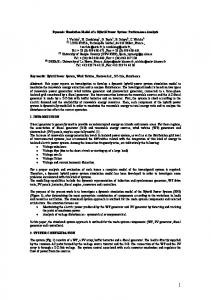
Efficient hybrid simulation of autotuning PI controllers Alberto Leva, Marco Bonvini∗ Dipartimento di Elettronica e Informazione, Politecnico di Milano Via Ponzio 34/5, 20133 Milano, Italy {leva,bonvini}@elet.polimi.it ∗ PhD student at the Dipartimento di Elettronica e Informazione
Abstract Autotuning methods are typically conceived as procedures, thus need simulating as digital blocks. However, when no autotuning is in progress, it is far more efficient to represent the tuned controller as a continuous-time system, to exploit variable-step integration. This manuscript presents the first nucleus of a Modelica library of autotuning controllers, where the problem just mentioned is tackled explicitly. The focus is here restricted to the PI structure, but the presented ideas are general. Keywords: Autotuning; PI control; hybrid systems’ simulation.
1
Introduction
It is universally acknowledged that PI and PID regulators significantly contribute to form the backbone of industrial controls [5, 3]. Also, in many applications and especially in recent years, their automatic tuning is of paramount importance for a quick system setup and an easy maintenance. As a result, an impressing quantity of autotuning rules can be found in the literature, see e.g. the vast review [17]; analogously, a large and steadily increasing number of industrial application and products are available, as testified by works such as [15]. Apparently, therefore, the simulation of PI(D) autotuners is a very interesting topic, for at least two reasons. From the standpoint of the analyst who performs system-level simulation studies, for example in a view to ease and speed the commissioning of a plant, autotuning is precious to reduce the time needed to parametrise the included regulators, that are often quite numerous. From the point of view of engineer who develops autotuning controllers, conversely, the possibility of testing a product (with a quasi-replica code representation) on realistic simulation models is
equally precious, since doing so allows to assess a priori its correct behaviour in the whole class of application it is intended for. However, in a view to achieve efficient simulation, the presence of autotuning regulators poses a relevant issue. The problem is that autotuners are typically conceived as digital blocks, and for the sake of correctness and precision, so need to be their models. On the other hand, when no autotuning is in progress, the regulator behaves as a fixed-parameter dynamic system, thus it is far more convenient to represent it in the continuoustime domain, so as to exploit variable-step integration. In such a context, this manuscript presents the first nucleus of a Modelica library of autotuning controllers, and concentrates on their hybrid representation, encompassing a continuous-time model of the controller, and a digital model of the autotuning part. After a brief theoretical review, a general structure for the necessary Modelica models is proposed as the main contribution, and an application that refers to a relay-based PI autotuner is presented. Simulation examples show the efficiency advantages of the presented hybrid representation with respect to a fully digital one.
2
Theoretical background
This work, although (as can be guessed) the proposed ideas are general, limits the scope to relay-based autotuning, and considers a one-degree-of-freedom PI written in the Laplace transform domain as the errorto-control transfer function � � 1 R(s) = K 1 + , (1) sTi where K is the gain and Ti the integral time. The basic principle of relay-based autotuning was introduced in [1], and then developed in [2, 8, 4, 16, 9] and many other papers; a survey on the matter, for the interested reader, can be found in [21].
In extreme synthesis, the idea is to lead the controlled system to a limit cycle by substituting the controller to be tuned with a relay, as shown in figure 1.
Figure 2: One-point identification with relay plus inFigure 1: Basic scheme for relay-based (PI) autotuntegrator feedback. ing. Once said condition is established, by measuring the period and amplitude of the induced controlled variable’s oscillation and by resorting to the well known describing function approximation, it is possible to esb jωox ) = Pox e jϕox of the process fretimate one point P( quency response P( jω), where ωox is the mentioned oscillation frequency. Then, to tune the PI, a point L is chosen that the open-loop frequency response L( jω) = R( jω)P( jω) has to contain, and the two parameters of the regulator R(s) are found by solving the complex equation R( jωo x)Pox e jϕox = L.
(2)
A widely used specification in relay-based PI autotuning is the closed-loop phase margin ϕm , which is enforced in a straightforward way by forcing L( jω) to cross the unit circle, at frequency ωox , in the point L = e j(ϕm −π) , with ϕm in radians. In this work, a slight variant of the scheme shown in figure 1 is used, where the relay is hysteresis-free, or has so small a hysteresis to allow the real negative semiaxis to be considered its critical point locus, and there is an integrator cascaded to it. Doing so causes the oscillation to occur at the frequency where the phase of P( jω)/( jω) is −π, i.e., that of P( jω) is −π/2. The situation is illustrated in figure 2, where M denotes the frequency response magnitude of P(s)/s at frequency ω − ox In this case, some computations omitted for brevity lead to determine the magnitude of P( jω) at the oscillation frequency ωox as Pox =
π 2A , 8D
(3)
−π/2 is a convenient choice, since a PI regulator can only introduce a phase lag: the desired phase margin ϕm is in fact obtained by drawing from (2) the two real equations for magnitude and phase, whence the simple tuning rules Ti =
tan(ϕm ) , ωox
K=
tan(ϕm ) p , Pox 1 + tan2 (ϕm )
(4)
that are used for the PI autotuner presented later on in this work. Many variants of (4) exist in the literature, see e.g. [18, 20] or the so called “contextual autotuning” recently proposed in [12]. Moreover, the same tuning principle is applicable to the PID, and also to more complex regulator structure, possibly detecting and employing several points of P( jω). The results shown here can be easily extended to any such case.
3
Modelica implementation
This section presents two Modelica realisations (the first fully digital, the second hybrid) of the considered autotuning methodology. In both cases, the icon of the resulting block is that of figure 3.
Figure 3: Modelica icon of the autotuning PI controller.
The block inputs are the set point and the process variable, plus a boolean one, a pulse on which initiates where A is the amplitude of the controlled variable’s the autotuning procedure; the output is clearly the conpermanent oscillation, and D the relay swing. Select- trol signal. The initial values for K and Ti , as well as ing the process frequency response point with phase the required phase margin, are provided as parameters.
In both realisations, with reference to figure 1 and the relationships introduced above, the autotuning procedure is composed of the following steps: 1. start with the controller in PI mode; 2. when the AT pulse is received, (a) initialise the relay plus integrator control, (b) connect it to the process, (c) and wait for a permanent oscillation; in the quite simple procedure presented here, an oscillation is considered permanent when the difference between its period and that of the previous one is less than a percent defined as parameter, while - for the sake of safety in the face of possible outliers - a certain number of oscillations, defined as a parameter too, is counted unconditionally before proceeding; 3. when a permanent oscillation is detected, compute its frequency, and by means of (3) determine the corresponding process frequency response magnitude (the phase is −π/2); 4. apply (4) to tune the regulator, and finally switch back to PI mode. It is worth noticing that any industrial realisation would be more articulated than those illustrated in the following. For example, some logic would need introducing to abort the procedure in the case of unexpected and/or possibly harmful system behaviours, a confirmation should be requested to the operator in order to accept or decline the proposed parameters prior to updating the PI, and so forth. Such features are however omitted here since they are lengthy to discuss in the necessary detail, and substantially inessential for the purpose of this work.
3.1
Fully digital version
Based on the procedure sketched above, it is quite simple to write a digital Modelica model like that reported below, together with some comments that should be explicative enough compatibly with space limitations. model ATPIrelayNCdigital import Modelica.Constants.*; parameter Real K0 = 1 parameter Real Ti0 = 10 parameter Real slope = 0.1 parameter Real permOxPerc = 5 parameter Real pm = 45 parameter Real CSmax = 1 parameter Real CSmin = 0 parameter Integer nOxMin = 3 parameter Real Ts = 0.1 protected
"Initial K"; "Initial Ti"; "relay integrator gain (control slope)"; "% diff to take oscillations as equal"; "reqd phase margin in degrees"; "upper control saturation value"; "lower control saturation value"; "oxs to wait for unconditionally"; "sampling time";
discrete Boolean UP; // relay is in the up state discrete Real lastToggleUp; // instant of last toggle to up discrete Real period; // measured ox period discrete Real wox; // measured ox frequency discrete Real Pox; // measured process mag at wox discrete Real rPVmax // service variables to measure the discrete Real rPVmin; // min and max values of the process discrete Real rCSmax; // variable and the control during discrete Real rCSmin; // oscillations discrete Real K; // PI gain discrete Real Ti; // PI integral time discrete Real e; // error (Sp-PV) discrete Real CSp; // proportional part of CS discrete Real CSi; // integral part of CS discrete Integer nOx; // ox counter discrete Integer iMode; // mode: 0 is PI, 1 autotuning Modelica.Blocks.Interfaces.RealInput SP; Modelica.Blocks.Interfaces.RealInput PV; Modelica.Blocks.Interfaces.RealOutput CS; Modelica.Blocks.Interfaces.BooleanInput ATreq; algorithm when initial() then iMode := 0; K := K0; Ti := Ti0; end when; when ATreq==true then iMode:=1; end when; when sample(0,Ts) then e := SP-PV; if iMode==0 then // PI mode CSp := K*e; CSi := pre(CSi)+K*Ts/Ti*e; CS := CSp+CSi; if CS>CSmax then CS:=CSmax; end if; if CSrPVmax then // record max and min for PV and CS rPVmax := PV; end if; if PVrCSmax then rCSmax := CS; end if; if CS0 and nOx>=nOxMin and abs(period-pre(period))/period < permOxPerc/100 then iMode := 0; wox := 2*pi/period; Pox := pi^2*(rPVmax-rPVmin)/8/(rCSmax-rCSmin); Ti := tan(pm/180*pi)/wox; K := tan(pm/180*pi)/(Pox*sqrt(1+(tan(pm/180*pi))^2)); CSi := CS-K*Ts/Ti*e; // re-initialise the PI after AT end if; rPVmax := PV; rPVmin := PV; rCSmax := CS; rCSmin := CS; nOx := nOx+1; end if; end if; end when; end ATPIrelayNCdigital;
linFBout the output of the feedback block, added in the diagram to the term Ke. When everything is digital, things are simple, and the Given all that, the Modelica model of the hybrid auonly issue to care about is to correctly manage the regtotuning PI is shown in the listing below. ulator tracking while the relay is driving the control signal so as to achieve the required permanent oscil- model ATPIrelayNCmixedMode import Modelica.Constants.*; lation. If conversely one wants to represent the con- // ... same parameters as the fully digital version ... Integer iMode; troller as a continuous-time system, it is necessary to Real K; Real Ti; suitably coordinate it with the digital procedure. Real satIn; Real linFBout(start=0,stateSelect=StateSelect.always); The solution adopted here can be summarised as fol- Real CSpi; Real CSat; lows. First, implement the controller in the desired discrete discrete Boolean AT; Boolean UP; form (here, for consistence with the digital case, an an- discrete discrete Real rPVmax; discrete Real rPVmin; tiwindup PI was chosen) as differential and algebraic discrete Real rCSmax; Real rCSmin; equations. Then, realise the autotuning procedure as discrete discrete Real lastToggleUp; Real period; a digital algorithm, including the control computation discrete discrete Real wox; discrete Pox; during that procedure, exactly as it was in the fully dig- discrete Real Integer nOx; // ... same connectors as the fully digital version ... ital case. Finally, manage the autotuning request event equation Continuous-time antiwindup PI by (a) setting a flag that selects the control output to be // satIn = K*(SP-PV)+linFBout; = Ti*der(linFBout)+linFBout; that coming from the equations or the algorithm, de- CSpi CSpi = noEvent(max(CSmin,min(CSmax,satIn))); // Output pending on the mode, and (b) initialising the algorithm if iMode==0selection or iMode==1 then // 0, PI or 1, AT init CS = CSpi; output to the last equation output. Analogously, manelse // 2, AT run CS = CSat; age the autotuning termination by resetting the above end if; flag, and reinitialising the equation-based controller algorithm // Autotuning procedure state to match the last algorithm output. when initial() then K := K0; The only (small) disadvantage of such a solution is Ti := Ti0; AT := false; that the equation-based controller stays in place during end when; when ATreq and sample(0,Ts) then // Turn on AT when required the autotuning phase. However the resulting overhead if not AT then AT := true; // set AT flag on is generally very limited, given the invariantly simple iMode := 1; // set next mode to AT init end if; structure of the controller, while there is a gain in terms end when; and iMode==1 and sample(0,Ts) then // AT init mode of simplicity with respect to possible alternative solu- when AT iMode := 2; // set mode to AT run CSat := pre(CSpi); tions attempting to avoid said overhead. UP := false;
3.2
3.3
From fully digital to hybrid
Hybrid version
The PI for this realisation is implemented in antiwindup form, i.e., as the block diagram of figure 4.
Figure 4: Block diagram of the used continuous-time antiwindup PI. That scheme corresponds in Modelica to the equations satIn = K*(SP-PV)+linFBout; CSpi = Ti*der(linFBout)+linFBout; CSpi = noEvent(max(CSmin,min(CSmax,satIn)));
where CSpi is the control signal in PI mode (u in figure 4), satIn the input of the saturation block, and
period := 0; wox := 0; Pox := 0; rPVmax := pre(PV); rPVmin := pre(PV); rCSmax := CSat; rCSmin := CSat; lastToggleUp := time; nOx := 0; end when; when (iMode==1 or iMode==2) and not AT and sample(0,Ts) then // AT shutdown; iMode := 0; reinit(linFBout,CSat); // re-initialise the continuos-time PI end when; when AT and iMode==2 and sample(0,Ts) then // AT run mode if UP==false and PVSP then UP := false; end if; if UP==true then CSat := CSat + slope*Ts; else CSat := CSat - slope*Ts; end if; if PV>rPVmax then // record relay id max and min for PV and CS rPVmax := PV; end if; if PVrCSmax then rCSmax := CSat; end if; if CSat0 and nOx>=nOxMin and abs(period-pre(period))/period < permOxPeriodPerc/100 then AT := false; wox := 2*pi/period; Pox := pi^2*(rPVmax-rPVmin)/8/(rCSmax-rCSmin); Ti := tan(pm/180*pi)/wox; K := tan(pm/180*pi)/(Pox*sqrt(1+(tan(pm/180*pi))^2)); end if; rPVmax := PV; rPVmin := PV; rCSmax := CSat; rCSmin := CSat; nOx := nOx+1; end if; end when; end ATPIrelayNCmixedMode;
Notice the presence of some noEvent clauses. In principle they can be omitted, but leaving them in slightly reduces the computational burden and, above all, is consistent with the operation of real-world autotuners, where inputs are typically acquired only at the beginning of a sampling period. Also, observe how the proposed structuring can be quite easily generalised, including different tuning rules, different types of process stimulation (e.g., stepinstead of relay-based) and different controller structures, since the presence of the autotuning algorithm does not modify in any sense the controller equations.
4
Simulation examples
In this section, two simulation examples are reported, to show the advantages yielded by the proposed autotuner models, and to verify their correct behaviour in realistic situations.
4.1
Example 1
This example aims at illustrating the correctness of the hybrid realisation, and its usefulness in terms of simulation efficiency. The Modelica scheme used for the example is that of figure 5, where the ATPI block is the fully digital or the hybrid autotuning PI, alternatively.
Figure 5: Modelica scheme for simulation example 1.
The process under control is described by the transfer function 1 (5) P1 (s) = (1 + s)3 and the autotuning PI, in both the fully digital and the hybrid versions, is employed with a sampling time Ts of 0.1s, first leading the loop to steady state with a lowperformance initial PI, then performing the autotuning operation with a required phase margin of 45◦ , and finally testing the so obtained PI with a set point and a load disturbance step, introduced respectively by the step sources SP and LD in figure 5. Figure 6 shows the results, proving that the two realisations are de facto identical as for their outcome (in both cases, for example, the tuned PI has K = 1.078 and Ti = 1.751). On the other hand, however, the number of simulation steps required by the system with the hybrid autotuner in the 240s presented run is 3908, versus the 24007 of the system with the fully digital one. With so simple a process this does not turn into a significant reduction of the simulation time, but with more realistic a model of the controlled object, said advantage would be evident.
4.2
Example 2
This example shows the presented autotuner at work on a (slightly) more realistic example, namely the speed control of an axis, the model of which is built with standard Modelica blocks (with the sole exception of a noise generator) and is shown in figure 7. Three tuning operations are performed, with three different values of the required phase margin, namely 40◦ , 60◦ , and 80◦ . Figure 8 shows the tuning results, obtained with the hybrid version of the autotuner (of course the fully digital one produces the same outcome). For brevity only the final part of the performed simulations is shown, when the PI is already tuned and the closed-loop system behaviour is tested by applying a set point step. As can be seen, even in the presence of (reasonably) noisy measurements, the autotuning PI behaves correctly. It must be noticed that with the used tuning approach, the control system’s cutoff frequency is dictated by the relay plus integrator experiment, as it clearly becomes ωox . For that reason, the relationship between the required phase margin and the shape of the obtained closed-loop transients, or even basic characteristics such as the maximum overshoot, is difficult to characterise in a formal way. Incidentally, this is especially true in the presence of resonances above the cutoff, which is typical of mechanical systems.
Figure 6: Closed-loop transients in simulation example 1. Nonetheless, the prescribed phase margin is achieved, and in any case the mentioned difficulty is inherent to the employed autotuning approach, not to its Modelica representation. The interested reader can find in [8] a discussion on this matter.
Figure 7: Model of the axis used in simulation example 2.
5
Some more words on the proposal usefulness
It was suggested above, as one of the motivations for this work, that a Modelica library of autotuners is useful to quickly set up the control system of a plant, or at least the part of it that is composed of PI(D) loops, and to verify the correct behaviour of a new autotuner by applying it in simulation to a benchmark set of models, conveniently chosen so as to represent the whole variety of applications where the new product is meant to be used. After looking at the examples, and taking a more research-related point of view, at least one more use-
fulness can however be foreseen for such a library, and the underlying model structuring. Apologising in advance for the number of remarks to report prior to reaching the main point, the matter can be explained as follows. In the first place, as can be noticed e.g. from the extensive review [17], establishing a taxonomy of tuning methods, also if the scope is restricted to a single controller structure, is far less trivial than one may expect. Even more difficult is to set up a comparative analysis of such methods, basically because in the literature, when proposing and discussing a method, the process stimulation and information gathering phase is seldom accounted for. As shown in works like [14], comparisons between different tuning methods can be reversed by simply modifying the way in which the process is stimulated. For the sake of completeness, it is worth observing that relay-based rules are the less keen to incur in that problem, since there is virtually no ambiguity on how process information is obtained and use with respect for example to the step-based identification of a fixed-order model, that can be carried out in a variety of manners, but nevertheless the problem exists, and needs addressing. The absence of a taxonomy like that just envisaged is felt in the applications as an important open problem, see e.g. [11], because it makes it difficult to decide a priori which tuning rule is best suited for the particular problem at hand. In the opinion of the authors, the fact that a tuning method “sometimes works satisfactorily and sometimes does not”, with no apparent reason, is a major reasons for the resistances that autotuning still encounters in some applications. It is
Figure 8: Tuning results in simulation example 2. by definition possible to decide which rule (in a given and wide enough set) is the best for a given problem a posteriori, by simply applying all the rules in the set and examining the results, but this is clearly infeasible in practice. As a result, most tuning rules are discussed “in nominal conditions”, i.e., making some structural assumptions on the process dynamics and performing the analysis under the hypothesis that the real process adheres to said assumptions [3]. Some attempts were made to circumvent the problem by means of the robust control theory, but this requires information on the class of processes to which the one under control belongs, and no matter how such a class has to be characterised, no single experiment can provide the necessary information. Attempts were also made to bring in the “identification for control” theory [6, 7], but unfortunately in many cases technological limitations do not permit to apply process inputs with the necessary excitation characteristics, and leave little (if any) room for “experiment design” as meant for in that theory. For the problem just sketched, the presented library offers (part of) a solution. In fact, if evaluating a set of control rules a posteriori is infeasible in practice, it is not in simulation. Having in mind the type of application to be addressed (thermal, mechanical, and so forth), one can set up an enormous set of cases, test each considered rule on each case, and draw from such a simulation campaign the information required to set up a selection mechanism. In fact there are plenty of techniques to create such a mechanism, from interpo-
lation to soft computing [13, 10], and what is typically missing is precisely the data. On a similar front, when introducing a new tuning rule, the proposal is significantly strengthened if some idea is provided on how it will behave when coupled to realistic process experiments. Providing such information requires a lot of additional work with respect to the typical analyses performed in the literature, that are most frequently based on linear models, because in that domain is autotuning typically treated, and only the linear framework allows for powerful methods that do not require simulation. As noticed e.g. in [19], however, the used models are frequently inadequate to examine the behaviour of an autotuner in the large, and therefore the mentioned analyses are sometimes confuted by experience, thereby further hindering a wide adoption of autotuning. Needless to explain why and how, the availability of a library like that presented here can help solve also this problem.
6
Conclusions and future work
The problem of simulating autotuning industrial controllers in Modelica was addressed, with the specific aim of obtaining efficient models. To this end, the controller is represented as a continuous-time system, while the autotuning procedure is realised as an algorithm. The proposed model structuring thereby allows to separate the two main parts of an autotuner clearly, preserving the simulation speed yielded by continuous-time control blocks, and replicating the autotuning software precisely.
As shown by the reported examples, and a number of other ones not reported here for space reasons, the so obtained simulation models are very precise if compared to fully digital ones, that certainly represent industrial implementation more closely, but oblige to pay for said fidelity in terms of simulation speed. In this work, the focus was restricted to relay-based PI autotuning based on a single point of the process frequency response. It is however clear that the presented structuring is totally general, with respect to both the controller structure, the type of process stimulation, the tuning rules, and all in all the overall tuning procedure, inclusive of the logic needed to control the tuning operation. Future research will thus explore all those extensions, leading to a complete Modelica library of autotuning controllers, including different tuning rules and excitation procedures, and possibly addressing not only single controller blocks, but also the most frequently used control structures.
[9] A. Leva. Simple model-based PID autotuners with rapid relay identification. In Proc. 16th IFAC World Congress, Praha, Czech Republic, 2005. [10] A. Leva and F. Donida. Normalised expression and evaluation of pi tuning rules. In Proc. 17th IFAC World Congress, Seoul, Korea, 2008. [11] A. Leva and F. Donida. Quality indices for the autotuning of industrial regulators. IET Control Theory & Applications, 3(21):170–180, 2009. [12] A. Leva, S. Negro, and A.V. Papadopoulos. PI/PID autotuning with contextual model parametrisation. Journal of Process Control, 20(4):452–463, 2010. [13] A. Leva and L. Piroddi. Model-specific autotuning of classical regulator: a neural approach to structural identification. Control Engineering and Practice, 4(10):1381–1391, 1996.
References
[14] A. Leva and L. Piroddi. On the parameterisation of simple process models for the autotuning of [1] K.J. Åström and T. Hägglund. Automatic tuning industrial regulators. In 26th American Control of simple regulators with specifications on phase Conference (to appear), New York (USA), 2007. and amplitude margins. Automatica, 20(5):645– 651, 1984. [15] Y. Li, K.H. Ang, and C.Y. Chong. Patents, software, and hardware for PID control—an [2] K.J. Åström and T. Hägglund. Industrial adaptive overview and analysis of the current art. IEEE controllers based on frequency response techControl Systems Magazine, pages 42–54, februniques. Automatica, 27(4):599–609, 1991. ary 2006. [3] K.J. Åström and T. Hägglund. Advanced PID [16] W.L. Luyben. Getting more information from control. Instrument Society of America, Rerelay feedback tests. Industrial & Engineering search Triangle Park, NY, 2006. Chemistry Research, 40(20):4391–4402, 2001. [4] A. Besançon-Voda and H. Roux-Buisson. An- [17] A. O’Dwyer. Handbook of PI and PID controller other version of the relay feedback experiment. tuning rules. World Scientific Publishing, SingaJournal of Process Control, 7(4):303–308, 1997. pore, 2003. [5] R.C. Dorf and H. Bishop. Modern control sys- [18] R.C. Panda and C.C. Yu. Analytical expressions tems. Addison-Wesley, Reading, UK, 1995. for relay feed back responses. Journal of Process Control, 13:489–501, 2003. [6] M. Gevers. Identification for control: from the early achievements to the revival of experiment [19] F.G. Shinskey. Process control: as taught versus design. European Journal of Control, 11(4– as practiced. Industrial & Engineering Chem5):335–352, 2005. istry Research, 41(16):3745–3750, 2002. [7] H. Hjalmarsson. From experiment design to [20] T. Thyagarajan and C.C. Yu. Improved autotunclosed-loop control. Automatica, 43:393–438, ing using the shape factor from relay feedback. 2005. Ind. Eng. Chem. Res., 43:4425–4440, 2003. [8] A. Leva. PID autotuning algorithm based on re- [21] C.C. Yu. Autotuning of PID controllers: relay feedback approach. Springer-Verlag, London, lay feedback. IEE Proceedings-D, 140(5):328– 1999. 338, 1993.