Especially interesting here is the comparison between the two David models at .... J. S. Vitter, âExternal memory algorothms and data structures,â in External ...
Efficient view-dependent out-of-core visualization Michael Guthe, Pavel Borodin and Reinhard Klein University of Bonn, Institute of Computer Science II R¨omerstraße 164, 53117 Bonn, Germany ABSTRACT Hierarchical levels of details (HLODs) have proven to be an efficient way to visualize complex environments and models even in an out-of-core system. Large objects are partitioned into a spatial hierarchy and on each node a level of detail is generated for efficient view-dependent rendering. To ensure correct matching between adjacent nodes in the hierarchy care has to be taken to prevent cracks along the cuts. This either leads to severe simplification constraints at the cuts and thus to a significantly higher number of triangles or the need for a costly runtime stitching of these nodes. In this paper we present an out-of-core visualization algorithm that overcomes this problem by filling the cracks generated by the simplification algorithm with appropriately shaded fat borders. Furthermore, several minor yet important improvements of previous approaches are made. This way we come up with a simple nevertheless efficient view-dependent rendering technique which allows for the natural incorporation of state-of-the-art culling, simplification, compression and prefetching techniques.
1. INTRODUCTION Polygon models generated by scientific or engineering visualization and especially from 3D scanners exceed the capability for interactive rendering on standard graphics hardware. Furthermore it is not uncommon that these models are several gigabytes in size and thus also exceed the amount of main memory available in a common PC. Many acceleration techniques have been developed to render complex models at interactive frame rates. They include visibility culling, simplification and image based or sampled representations. Visibility culling only works good for models with high depth complexity and image based methods tend to produce more popping artifacts than simplification. Therefore the simplification approaches are most promising for general complex datasets. Early simplification techniques can generally be divided into two approaches, static and view-dependent,1 where both have their advantages and drawbacks. View-dependent simplification represents the geometry as split/collapse operations that are only locally dependent. Therefore, they can be applied depending on the position of the viewer to generate an approximation that results in the same screen space error everywhere on the model. Furthermore, the view-dependent LOD allows a smooth transition between frames since split/collapse operations approximate geomorphing.1 In contrast to this, static levels of detail are representations generated from the original model, that have the same geometric error on the whole model. Since no split/collapse operations are stored, no smooth transitions between different LODs are possible. A recent extension of static level of detail are the hierarchical LODs that are build upon a bounding box hierarchy for more effective simplification. To generate coarser levels of detail whole subbranches of the bounding box hierarchy are combined to a single object and simplified. If spatially large objects are partitioned hierarchically, HLODs are an approximation of view-dependent simplification. When it comes to out-of-core simplification, static HLODs are most commonly used because view-dependent simplification is too costly for scenes containing several hundred million triangles. At the cuts through spatially large objects however, the subparts cannot be simplified without introducing cracks in the model. √ This restricts the simplification of these objects to produce at least O( n) triangles where n is the original number in the subpart. On the other hand using runtime stitching requires much CPU power and therefore a multiprocessor system or a cluster is needed. E-mail: {guthe,borodin,rk}@cs.uni-bonn.de
To overcome this problem we use a crack filling algorithm that entirely works on recent graphics hardware and thus leaves the CPU power for decompression and culling techniques. It reduces the number of triangles to approximately O(k), where k only depends on the simplification error and thus on the desired size of the LOD on screen. Since the cracks have to be closed by the simplifier during the construction of HLODs for inner nodes we use a simplifier that efficiently performs topological simplification. Additionally we present an efficient and simple motion prediction algorithm for a more efficient geometry prefetching and thus reduction of misses during rendering. The main features of our algorithm are: • • • •
Interactive high fidelity out-of-core visualization of complex scenes containing tens of million triangles. Screen space error of less than 12 pixel compared to the original model. Filling of cracks introduced due to independent simplification of subparts entirely on graphics hardware. Prioritized prefetching with a simple motion prediction based on natural movement to reduce the number of misses. • Reduced number of triangles in each node compared to previous HLOD rendering algorithms like Ref. 2, 3. • Optimized geometry with respect to rendering time an AGP bus load.
2. RELATED WORK In this section we give a brief overview of related work in the area of large model and out-of-core visualization.
2.1. Large Model Visualization Many methods have been developed for the visualization of large models. They are based on the three main approaches geometric simplification, visibility culling and image based representations. Geometric simplification algorithms generate an approximation of the original model with reduced number of primitives. A recent survey of simplification algorithms can be found in Ref. 4. They can be classified as either dynamic (view-dependent) or static (view-independent), although, as shown in Ref. 3 static HLODs generated by partitioning approximate view-dependent simplification. Visibility culling algorithms try to quickly determine possibly visible and definitely invisible (culled) objects. There are three general methods to determine and remove invisible parts of the scene. The first is view frustum culling which removes all objects outside the actual view frustum. The second is backface culling that removes all polygons facing away from the current view position. If normal cones5 are used, whole objects or subtrees of a scene graph can be removed from rendering. The third approach is occlusion culling where objects are removed from the scene that are hidden behind other objects. Ref. 6 gives a good overview of different occlusion culling approaches. Image based representations use impostors to replace distant objects with previously rendered images.7–11 In cell based approaches they can be combined with geometric simplification as in Ref. 7.
2.2. Out-of-Core Algorithms In computational geometry and related areas a lot of work has been spent on so called out-of-core or external memory algorithms.12, 13 Based on the spatial subdivision of architectural models a real-time memory management algorithm to swap objects in and out of memory was developed by Funkhouser et al.14, 15 and Aliaga et al.7 developed a system for interactive rendering of complex models than can easily be partitioned into cells. However there is no good algorithm known for partitioning a general model into such cells. Furthermore, the image based methods used in this work tend to produce severe popping artifacts. A number of out-of-core simplification algorithms for large models have been developed16–20 that can be used to generate static levels of detail. An out-of-core simplification algorithm for view-dependent simplification was developed by El-Sana and Chiang21 and tested for models with a few hundred thousand triangles. Although viewdependent simplification22–25 generates less triangles to be rendered and works well for spatially large objects it has a significant overhead during visualization. Instead of performing calculations at nodes inside a scene graph
only it has to query every active vertex or edge of all visible objects. Furthermore, since the geometry of the objects changes frequently, it has to be sent to the graphics card at almost every frame shifting the bottleneck from fill rate limitations to bus speed. A few out-of-core visualization methods including rendering of large unstructured grids26 and isosurface extraction27, 28 have been developed. In Ref. 29, 30 application controlled segmentation and paging methods for the out-of-core visualization of computational fluid dynamics data were presented. A number of techniques like indexing, caching and prefetching31, 32 were developed to increase the performance for large environment walkthrough applications. Recently an out-of-core rendering algorithm33 was presented using hierarchical levels of detail.3
3. OVERVIEW In this section we give an overview of our visualization algorithm that is composed of level of detail generation, crack filling, culling and memory management. Since a general scene graph (if provided with the scene) may not be optimized for rendering, culling and HLOD generation, we ignore it and build a spatial axis aligned bounding box hierarchy. In contrast to previous approaches we subdivide the whole scene with an octree to create this hierarchy. An octree has the advantage that it is one of the most efficient spacial subdivisions for numerous culling techniques. The octree can only be used efficiently for subdivision since our algorithm does not require the geometry to exactly fit together between two adjacent HLODs in contrast to Ref. 33. Therefore, no constraints preventing efficient simplification would need to be minimized. Details of the HLOD generation are discussed in section 4 and a detailed description on the culling techniques applied is given in section 6.2 To fill the cracks between adjacent HLODs fat borders are rendered along the cuts of each inner HLOD node. Therefore the borders of the simplified geometry along a cut are stored together with the triangles on disk. When rendering a HLOD object, the fat borders are drawn using an algorithm we developed for view-dependent NURBS rendering34 which entirely runs on the graphics hardware to conceal the cracks. Section 5 shortly describes this technique and the modifications necessary for its adaption to HLODs in detail. To reduce latency when new geometry needs to be loaded from disk, we use a prefetching algorithm that runs parallel to the rendering thread. In contrast to previous prefetching techniques we estimate the likeliness of the geometry to be rendered not only using its approximation error and therefore the distance the camera has to travel, but also the angle by which it has to rotate. The geometry file format is described in section 4.4 and a detailed description of the prefetching algorithm can be found in section 6.3.
4. HLOD GENERATION In this section we describe the details of our method to generate HLODs. To prevent material changes inside a node that are very costly, especially when using textures, first all objects with the same material are clustered into a single superobject. Then they are partitioned with an octree, hierarchically grouping subparts and simplifying them together. It generates a HLOD (or LOD at leaf nodes) for every node of the octree and stores them on disk. Since the size of each node on screen and therefore the number of triangles contained in its geometry should be in a given range, the approximation error � of the geometry in a node has to be enode res where res is a constant depending on the screen space error �screen and the desired edge length of a node on screen escreen . This constant screen is defined as res = e�screen , where escreen can be optimized for a specific PC system.
4.1. Overall Algorithm After the combination of all objects with the same material these superobjects are treated separately. Therefore, the subsequent algorithm is only described for one such object. The partitioning algorithm starts with the whole superobject in the root node of an octree. The object is partitioned by cutting the geometry of each inner node into eight subparts and storing them in its children if its geometry contains more than Tmax triangles. The partitioning is repeated until no node was cut. If no
geometry is contained in a node it is marked and not partitioned further. The out-of-core partitioning algorithm is described in section 4.2. After the partitioning the geometry contained in the leafs of the octree is stored on disk. Starting from the geometry of these nodes the HLOD hierarchy is build recursively from bottom to top with the following algorithm: • Gather the simplified geometry from all child nodes that are two levels below the actual node (or the original geometry if there is no HLOD at this depth). Its approximation error �prev is then the maximum error of the simplified geometry in these child nodes. • Simplify resulting geometry as long as the Hausdorff distance �h to the gathered geometry is less than �s = enode res − �prev , where enode is the edge length of the currents nodes bounding cube and res is the desired resolution in fractions of enode . • Store � = �h + �prev as approximation error in the current node. By using the children at two levels below the actual node instead of its direct children the simplified geometry contains less triangles, since the approximation of the real geometric error is better. This is due to the fact that the difference between the estimated geometric error � and the real geometric error �real is low, since: �real ≥ �s =
enode res
− �prev ≥
enode res
−
enode 4·res
=
3 enode 4 res
= 34 � and thus 34 � ≤ �real ≤ �.
Instead of this recursive out-of-core simplification it would also be possible to use a traditional out-of-core simplification algorithm to build the HLODs of inner nodes directly from the original geometry during the partitioning process. However, starting with the combination of already simplified geometry greatly reduces the computation cost and still leads to high quality drastic simplifications. This is due to the fact that the number of triangles in the gathered geometry remains almost constant independent from the depth of the actual node and therefore, the number of triangles in the base geometry of this part of the object. This means that the total simplification time depends only linearly on the number of leaf nodes and thus linearly on the number of triangles in the base geometry. During the simplification process the geometric error of each nodes geometry is stored along with the bounding box of the contained simplified geometry. Finally the geometry of each node is compressed and stored on disk. Additionally the skeleton of the scene graph containing the bounding boxes and the geometric error of the simplified geometry contained in each node, but not the geometry itself, is stored. The size of such a node in the scene graph skeleton if less than 100 bytes and a leaf node should contain several thousand triangles on average for efficient rendering. Therefore the size of this skeleton is only 10 MB for a scene containing 100 million triangles. Nevertheless in contrast to previous algorithms we do not keep the whole skeleton in memory. At the point where the depth of the skeleton reaches 5 (≤ 641 KB), the subtrees are stored on disk and only loaded on demand. For faster loading these subtrees only have a depth of three before they branch into different files again. During runtime the root skeleton and the 100 last recently used subtrees (≤ 791 KB) are kept in memory.
4.2. Out-of-Core Partitioning Since the whole geometry of a node does generally not fit into the main memory, the vertices and normals of the mesh are stored in blocks and swaped in and out from disk using a last-recently-used (LRU) algorithm. The indices of the triangles need not to be stored in memory and therefore, can be streamed from the geometry file of the node to the files of its children. This is accomplished by loading the actual triangle from the geometry file of the node, cutting it and then saving the generated triangles in the child geometry files. After the triangle is cut it is not needed any more. Therefore, only the actual triangle and the triangles generated from it are stored in memory. When first saving all triangles in the root node, the vertex normals are calculated. At each partitioning step every triangle is cut with the three planes dividing the node into its children and the resulting triangles are stored in the appropriate geometry files. When a triangle edge is cut, the normal of the new point is calculated by linear interpolation. Note that new vertices may have the same coordinates as existing vertices, but this is resolved when the whole tree is build. After partitioning the triangles of a node
and storing it in its children, the geometry file of this node is not used any more and is deleted. When the partitioning is complete new indices for the leaf node triangles are calculated and duplicate points are removed. The total complexity of the partitioning algorithm is O(n log n), since on each level of the octree all triangles need to be processed once.
4.3. Simplification of a Node Since we need to combine disjoint parts of the superobject during simplification, the simplifier needs to be capable of performing topological simplification in order to close the cracks introduced by the partitioning and independent simplification in previous stages of the recursion. Furthermore it has to be capable of simplifying the geometry up to a given geometric error (Hausdorff distance). For this reason we use the generalized pair contractions algorithm described by Borodin et al..35 This approach completely generalizes the vertex pair contraction operation introduced by Popovic and Hoppe36 and Garland and Heckbert37 by allowing contractions between a vertex and any other mesh simplex (vertex, edge or triangle) or between two edges. These technique allows to connect disjoint parts of the mesh already on the early stages of simplification.
Figure 1. Hierarchical simplification using only vertex pair contractions (left) and generalized pair contractions (right).
Figure 2. HLODs rendered for a specific view point (near the head). Note how the HLODs approximate the continuous viewdependent level of detail and the fat borders allow better simplification along cuts (left, fat borders not rendered) compared to Ref. 3 (right).
Since the hierarchical simplification introduces narrow cracks between disjoint surface regions, performing standard vertex pair contractions simplification on such data could have undesirable results (figure 1, left). Use of generalized pair contractions will resolve this problem by sewing disconnected parts together (figure 1, right). Generalized pair contractions. In Ref. 35 the vertex pair contraction is extended to the generalized pair contraction by introducing the new operations: vertex-edge, vertex-triangle and edge-edge contractions. In case of vertex-edge and vertex-triangle contractions the contraction vertex is contracted onto intermediate vertex which is created on the contraction edge or triangle. In case of edge-edge contraction two intermediate vertices are created on each contraction edge and then contracted together. These three operations perform no reduction, but increase the connectedness of the mesh. Error metrics. As a criterium for the choice of next contraction operation we use a modification of the quadric error metrics presented by Garland and Heckbert.37 All candidate contraction pairs are sorted in a priority queue according to the error that will arise after contracting them. The new position of a contraction vertex is chosen in order to minimize this error. Control over geometric error. Although the quadric error metrics are a fast technique, which provides good results, it does not deliver the precise geometric error. In our case this is a necessary requirement. Furthermore we need the possibility to simplify up to a given geometric error. Therefore, in addition to quadric error metrics
we use the Hausdorff distance between the original and the simplified meshes. It is done the same way as described by Hoppe23 and Klein et al..38 The combination of different error metrics is a tradeoff between speed and accuracy. Since the input and output number of triangles generally remain constant, the complexity of the simplification algorithm linearly depends on the number of nodes in the octree and therefore is O(n). Therefore the complete HLOD generation algorithm has a complexity of O(n log n). The whole partitioning and simplification algorithm are paralelized. In our examples we used eleven PCs in a network for these preprocessing steps.
4.4. Compression of Connectivity and Geometry It would lead to no benefit if the geometry would be stored as a sequence of simplification operations to construct 1 it from its children two levels below, since it contains only approximately 256 of their vertices and so the number of operations exceeds the number of vertices in the geometry by a factor of approximately 200. The indices are stored using one, two or four bytes depending on the number of vertices. In addition to the triangle strips, the edge loops needed for the fat borders are stored. We do not use the Edgebreaker compression algorithm,39 since triangle strips already provide a good compression and the computation cost for decompressing the connectivity is too large compared to the benefit due to reduced loading time. For faster rendering the geometry is send as triangle strips to the graphics card. This strips are generated using a fast striping algorithm40 and then stored on disk. The algorithm produces stripes of an average length of 6. Therefore, only 8 instead of 18 vertices need to be shaded and transformed. In the optimal case this doubles the frame rate. To compress the vertex positions the bounding cube of the octree node is stored and the vertex coordinates of its geometry are discretized relatively to the bounding cube. Since the geometry of inner nodes is an approximation and already associated with a geometric error � it does not make sense to store the vertex positions with a much higher precision. We spent one bit more than needed to encode with an error of � for node ). When the geometry of such a node rendered an error of � is projected to at inner nodes (e.g. 8 bit for � = e128 most the desired screen space error �screen . Therefore storing the vertices with an error of 2� projects on screen to at most �screen . Since we use a screen space error of 12 pixel this is at most 14 pixel and can thus be neglected. 2 The normals are discretized to 8 bit per coordinate, which does in general not lead to a loss if image quality. If we choose for example res = 128 the vertex coordinates as well as the normals require 3 × 8 bit and therefore 48 bit = 12 bytes instead of 48 bytes when using float or even 96 bytes with double values. Since the coordinates generally need much more space than the connectivity this reduces the file to almost a third of the original size even without additional compression techniques. Since we use huffman coding to compress the files we can round all bit lengths up to full bytes for faster decompression.
5. CRACK FILLING The gap filling algorithm conceals the cracks between adjacent HLODs introduced during the simplification by rendering appropriately shaded fat borders.34 This has the big advantage that the HLOD of a node can be replaced without changing anything in the geometry of adjacent nodes and therefore, only information for the new node has to be send down the AGP bus and the cracks are filled. The width, displacement and color of the fat borders are calculated every frame using the vertex program shown in figure 3. The input data for rendering the fat borders from the cutting and simplification stage consists of all edges along the cuts that need to be filled and the approximation error of the node. Since the fat border algorithm needs edge loops or at least edge strips, they are generated when the geometry is stored on disk. The edge loops or strips are constructed by starting an edge strip with the first boundary edge and adding adjacent boundary edges at the start and end of this strip until no adjacent edge is left. Then the next strip is started, again with the first remaining boundary edge. If all boundary edges are concatenated to edge strips the tangent vectors are calculated as described in Ref. 34 with the exception that if an edge strip does not start and end in the same vertex, only one tangent is generated at the start end end of the strip.
!!ARBvp1.0 PARAM mvp[] = {state.matrix.mvp}; PARAM mv[] = {state.matrix.modelview[0]}; PARAM param = program.local[0]; TEMP view, length, pos; # compute per vertex lighting ... # compute view direction
MUL view, {-1, -1, -1, 0}, mv[2]; DP3 length, view, view; RSQ length, length.x; MUL view, length, view; # move in view plane XPD pos, view, vertex.texcoord[0]; DP3 length, pos, pos; RSQ length, length.x;
MUL pos, length, pos; MAD pos, pos, param, vertex.position; # move away from viewer MAD pos, view, param, pos; # transform and project vertex ... END
Figure 3. Vertex program to render fat borders. The tangent vectors are stored as texture coordinates and the approximation error is given as local program parameter. si -1
si ti
vi 3
vi 2
vi1
vi 4 v i5 si -1
ti
vi 6
si -1
si
vi 3 vi 4
si
si -1
vi 2
vi1
ti
vi 6
ti
vi 5
si
Figure 4. Fat border accuracy against speed tradeoff. Using only two vertices instead of al six increases the rendering performance at the cost of lower accuracy of the fat borders.
Figure 5. Workflow of the parallel rendering and prefetching thread for a single processor system.
Figure 6. Angles θ and γ used for visibility prefetching: V represents the view frustum, B the bounding box and N the normal cone of the current node.
To speed up rendering, we only use the middle two of the generated fat border vertices, as shown in figure 4, instead of all six and thus adding two triangles to the node for each boundary edge at a cut. Since the edges along a cut between adjacent HLODs do not need to be preserved, the approximation of a view-dependent level of detail is better and less triangles need to be rendered. Figure 2 demonstrates this approximation and how the fat borders fill the cracks between adjacent HLODs.
6. RENDERING 41
For rendering we use the OpenSG scene graph which has a build in support for view frustum and occlusion culling. Since disk access and rendering are able to run almost in parallel even on a single processor system two threads are used. The first thread traverses the octree and then renders the scene. During rendering, the prefetching thread loads geoemetry using a priority queue described in section 6.3.
6.1. Scene Representation For scene graph traversal and culling a scene graph skeleton is kept in memory. This skeleton stores parent child relationships, the bounding box and error metric for each node. Furthermore, the normal cone, a pointer to the geometry (if in memory) and the status of the node are kept in this skeleton. The geometry is loaded on the fly into main memory when it is needed for rendering. A memory footprint size can be given to the visualization algorithm and we ensure that no more memory than specified is used by our method. The only restriction to this footprint size is that the root of the scene graph skeleton and of course the rendering buffers have to fit into this amount of memory.
6.2. Culling Techniques Additionally to the built-in view frustum and occlusion culling,42 we implemented backface culling using normal cones.5 For this, the normal cones of the child nodes are combined during the HLOD generation to calculate the normal cone of an inner node. To update the actual scene graph the skeleton is traversed and the following operation are performed:
• Backface culling: The normal cone of the node is checked with the view direction. If the normal cone is completely facing away from the viewer, scene traversal is stopped. • View frustum culling: The bounding box of the node is checked against the view frustum and traversal is stopped when it is outside. • Occlusion culling: The node is checked for occlusion using its bounding box. Again traversal is stopped if the node is occluded. • HLOD selection: If the error metric � of the node is at most the desired error �des the geometry is rendered and traversal is stopped. If the node is not already in memory, it has to be loaded. The desired error is calculated by projecting the screen space error �screen to the point on the bounding box of the node which is closest to the viewer. Note that the backface and occlusion culling are optional because they do not make sense for all scenes (e.g backface culling for scene with double sided triangles and occlusion culling for scenes with low depth complexity).
6.3. Memory Management We use a mutex lock to synchronize the rendering and prefetching thread when the view changes. Additionally this lock is used to prevent the prefetching thread from using up CPU power during scene graph actualization and culling. The workflow of the two threads is shown in figure 5. We use two priority queues Qload and Qremove to determine which nodes should be loaded from disk and which of the currently unused geometry nodes are not needed in consecutive frames and thus can be removed from memory. The priority p of a node in these queues represents the likeliness that a node will be rendered in the next frame. In contrast to previous approaches14, 33 we do not only use the projected error of a node as base for the likeliness and cut off all nodes outside an extended view frustum. Instead we calculate the minimum angle the viewer would need to rotate to be able to see the node and then use this angle to weight the likeliness depending of the movement of the viewer. To calculate the priority of a node the scene graph is traversed and the priority p for all inactive nodes is calculated by the following formula: ( � �des : �des < �node pdetail : visible �node , p= , α = max(θ, γ), pdetail = �parent : else pdetail · arccos α : culled �des,parent where θ is the angle between the view frustum and the bounding box of the node and γ the angle between the normal cone and the view plane if the node is backfacing, otherwise zero. For the 2d case this is shown in figure 6. As long as enough memory is available the node with the highest priority Nload is loaded from Qload . If not enough memory is available to load Nload , the node with the lowest priority Nremove from Qremove is removed, if its priority lower than that of Nload . If no more geometry can be loaded without violating this condition the prefetching is stopped. The priority queues have to be updated each time the scene graph traversal starts. Since the number of nodes is very high for complex scenes the priority is calculated by traversing the octree and traversal is stopped as soon as p < pstop for a given pstop (we use 0.5) and �des < �node . All nodes of the hierarchy not reached by this traversal are then assumed to have a priority of zero. Note that we do not use occlusion culling to calculate the priority of a note, because occlusion can change very abruptly between frames. To predict the motion of the viewer, we use the fact that natural movements are continuous up to at least the second derivative. We approximate this movement by quadratic functions using the view position and direction of the last three frames. Based on this movement we predict the view position and direction of the next frame to perform a more efficient prefetching. This leads to the following formula to estimate the position Pi+1 and direction d~i+1 in the next frame: ~vi − ~vi−1
Pj −Pj−1 tj −tj−1
=
~vi+1 − ~vi
with ~vj =
Pi+1 −Pi ti+1 −ti
=
P −Pi−1 2 tii −ti−1
Pi−1 −Pi−2 ti−1 −ti−2
d~∗i+1
=
~ −d ~i−1 d d~i + (ti+1 − ti ) 2 tii −ti−1 −
−
�
~i−1 −d ~i−2 d ~i−1 −d ~i−2 d
�
~vi+1
=
2~vi − ~vi−1
Pi+1
=
Pi + (ti+1 − ti ) 2
d~i+1
=
�
~∗ d i+1 ~∗ k kd i+1
Pi −Pi−1 ti −ti−1
−
Pi−1 −Pi−2 ti−1 −ti−2
�
Since we cannot predict the time ti+1 when the next frame will be displayed, we assume that ti+1 −ti =
ti −ti−2 . 2
This prediction works well as long as the user does not release the mouse button and thus performs an abrupt stop or starts to press a button while moving the mouse. The first case is no problem for our algorithm, since the geometry for the actual view position is already in memory. The second case cannot be solved by any movement prediction algorithm since there is no data available to predict the movement from, when the viewer does not perform movements. It is not necessary to perform a prefetching for the subtrees of the scene graph skeleton since they are already loaded during the geometry prefetching.
7. RESULTS We tested our system with different models (see table 1) from the Stanford Scanning Repository43 (Armadillo, Happy Buddha, Dragon and Lucy) and the Digital Michelangelo Project44 (David) on a 1.8 GHz Pentium 4 PC with 512 MB memory and an ATI Radeon 9700Pro. As parameters for the partitioning algorithm we chose a maximum number of triangles per node of Tmax = 1024 and a ratio of error to node size res = 256 (max. 128 pixel per node in image space). For rendering we set pstop = 0.5, �screen = 12 and 256 MB as memory footprint size. Model
#Triangles
Armadillo Dragon Happy Buddha David 2mm Lucy David 1mm
345.944 871.414 1.087.716 8.254.150 28.055.742 56.230.343
Original model (raw data) 11.9 MB 29.9 MB 37.3 MB 283.4 MB 963.2 MB 1.9 GB
HLODs (comp.) 5.0 MB 11.9 MB 16.9 MB 98.3 MB 365.3 MB 675.1 MB
Out-of-core
With cracks
In-core
82.8 / 28.0 95.1 / 43.0 86.8 / 49.0 107.3 / 50.0 82.4 / 33.0 107.6 / 49.0
86.7 / 30.0 99.7 / 43.0 91.1 / 52.0 110.8 / 53.0 86.5 / 35.0 110.7 / 54.0
85.3 / 29.0 100.1 / 54.0 88.6 / 51.0 n.a. n.a. n.a.
Table 1. Triangle numbers of models used for testing and their size on disk; average / minimum frame rates for different rendering algorithms.
Since the depth complexity of the models is low and occlusion culling has a significant overhead we only used view frustum and backface culling in our tests. The camera paths used for testing are rotations of the object and zooms to interesting parts. To evaluate the performance of our out-of-core rendering system we compare it to in-core rendering (if possible for the model) and to out-of-core rendering without crack filling. For the in-core rendering we load all geometry when the scene graph skeleton is loaded and do not start the memory management thread. The last three rows in table 1 show the frame rates for the tested models at a resolution of 1024 × 768. Especially interesting here is the comparison between the two David models at different reconstruction resolutions since we used the same camera path for them to show how excellent our method scales with the size of the input model. The marginal increase of the frame rate is due to the fact that less original geometry needs to be loaded for the larger model since more HLODs are available. The frame rates with and without fat borders are almost identical since the number of fat border triangles is low compared to the number of normal triangles. Of course the achieved frame rates depend on the velocity of the viewer. For the recorded natural movement of the object almost no misses occurred. Therefore, a reduction of the velocity does not lead to higher frame rates as approved by different tests. Figure 7 shows the frame rates and memory management statistics of the David statue in detail for a freehand movement of the model. The memory management statistics show the memory needed for the actual rendered geometry (visible bytes: black) the size of the prefetched geometry (bytes prefetched: green) amd the size of the geometry that was loaded during octree traversal (bytes missed: red). The memory management statistics show that the prefetching works very well and only few misses occurred during the movement. The algorithm provides a good balance between GPU and CPU load since the GPU load is almost 100% and the CPU load is 95% on average. Since only few geometry is replaced between frames the AGP bus load is low, leaving enough bandwidth for textures.
Figure 7. Frame rates for the out-of-core rendering and memory management statistics of the 1mm David statue.
8. CONCLUSION AND FUTURE WORK In this paper we presented a simple but efficient out-of-core visualization algorithm using hierarchical levels of detail and a crack filling algorithm running on graphics hardware. An intelligent out-of-core simplification technique, allowing vertex-edge, edge-edge and vertex-triangles collapses, allows to merge parts of different nodes in the hierarchy in such a way that gaps between adjacent parts are closed in a controlled manner. The number of triangles in each HLOD node generated by partitioning can be reduced further compared to previous approaches, since the triangles at cuts do not need to be preserved. Additionally we optimize the geometry for rendering and AGP bus transfer. The algorithm has been tested on various models ranging from a few megabytes to more than one gigabytes showing its ability to render highly complex scenes at interactive frame rates on consumer level hardware. Furthermore, the results show the excellent scalability. Currently we are working on the incorporation of normal maps into our algorithm. In the future we will extend our system to support user provided target frame rates and explore more complex motion prediction schemes for a more focused prefetching. An interesting topic would be to set up standard paths and velocities for reference objects for a better comparison of different out-of-core rendering techniques (especially point set rendering).
ACKNOWLEDGMENTS This work was partially funded by the BMBF under the project of OpenSG PLUS. We thank Marc Levoy and the Digital Michelangelo Project for providing us with the models.
REFERENCES 1. H. Hoppe, “Progressive meshes,” Computer Graphics 30(Annual Conference Series), pp. 99–108, 1996. 2. W. V. Baxter, A. Sud, N. K. Govindaraju, and D. Manocha, “Gigawalk: Interactive walkthrough of complex environments,” 2002. 3. C. Erikson and D. Manocha, “HLODs for faster display of large static and dynamic environments,” in ACM Symposium on Interactive 3D Graphics, 2000. 4. D. Luebke, “A developer’s survey of polygon simplification algorithms,” in IEEE CG & A, pp. 24–35, IEEE, May 2001. 5. L. A. Shirman and S. S. Abi-Ezzi, “The cone of normals technique for fast processing of curved patches,” Computer Graphics Forum 12(3), pp. 261–272, 1993. 6. D. Cohen-Or, Y. Chrysanthou, and C. Silva, “A survey of visibility for walkthrough applications,” 2000. 7. D. G. Aliaga, J. Cohen, A. Wilson, E. Baker, H. Zhang, C. Erikson, K. E. Hoff, T. Hudson, W. St¨ urzlinger, R. Bastos, M. C. Whitton, F. P. Brooks, and D. Manocha, “MMR: An interactive massive model rendering system using geometric and image-based acceleration,” in Symposium on Intercative 3D Graphics, pp. 199–206, 1999. 8. D. G. Aliaga and A. Lastra, “Automatic image placement to provide a guranteed frame rate,” in Siggraph 1999, Computer Graphics Proceeding, A. Rockwood, ed., pp. 307–316, Addison Wesley Longman, (Los Angeles), 1999. 9. P. W. C. Maciel and P. Shirley, “Visual navigation of large environments using textured clusters,” in Symposium on Interactive 3D Graphics, pp. 95–102, 211, 1995.
10. G. Schaufler and W. St¨ urzlinger, “A three dimensional image cache for virtual reality,” Computer Graphics Forum 15(3), pp. 227–236, 1996. 11. J. Shade, D. Lischinski, D. H. Salesin, T. DeRose, and J. Snyder, “Hierarchical image caching for accelerated walkthroughs of complex environments,” Computer Graphics 30(Annual Conference Series), pp. 75–82, 1996. 12. Y.-J. Chiang, M. T. Goodrich, E. F. Grove, R. Tamassia, D. E. Vengroff, and J. S. Vitter, “External-memory graph algorithms,” in Symposium on Discrete Algorithms, pp. 139–149, 1995. 13. J. S. Vitter, “External memory algorothms and data structures,” in External Memory Algorithms and Visualization, J. Abello and J. S. Vitter, eds., pp. 1–38, American Methemathical Society Press, Providence, RI, 1999. 14. T. A. Funkhouser, “Database management for interactive display of large architectural models,” in Graphics Interface ’96, W. A. Davis and R. Bartels, eds., pp. 1–8, Canadian Human-Computer Communication Society, 1996. 15. T. A. Funkhouser and C. H. S´equin, “Adaptive display algorithm for interactive frame rates during visualization of complex virtual environments,” Computer Graphics 27(Annual Conference Series), pp. 247–254, 1993. 16. F. Bernadini, J. Mittleman, and H. Rushmeier, “Case study: Scanning michelangelo’s florentine pieta,” 1999. 17. P. Cignoni, C. Montani, C. Rocchini, and R. Scopigno, “External memory simplification of huge meshes,” in IEEE Trans. on Visualization and Comp. Graph., to appear, 2003. 18. P. Lindstorm, “Out-of-core simplification of large polygonal models,” in ACM Siggraph, 2000. 19. P. Lindstorm and C. T. Silva, “A memory insensitive technique for large model simplification,” in IEEE Visualization, IEEE, 2001. 20. E. Shaffer and M. Garland, “Efficient adaptive simplification of massive meshes,” in IEEE Visualization, IEEE, 2001. 21. J. El-Sana and Y.-J. Chiang, “External memory view-dependent simplification,” Computer Graphics Forum 19(3), 2000. 22. J. El-Sana and A. Varshney, “Generalized view-dependent simplification,” Computer Graphics Forum 18, pp. 83–94, September 1999. ISSN 1067-7055. 23. H. Hoppe, “View-dependent refinement of progressive meshes,” Computer Graphics 31(Annual Conference Series), pp. 189–198, 1997. 24. D. Luebke and C. Erikson, “View-dependent simplification of arbitrary polygonal environments,” Computer Graphics 31(Annual Conference Series), pp. 199–208, 1997. 25. J. C. Xia, J. El-Sana, and A. Varshney, “Adaptive real-time level-of-detail based rendering for polygonal meshes,” IEEE Transactions on Visualization and Computer Graphics 3(2), pp. 171–183, 1997. 26. R. Farias and C. T. Silva, “Out-of-core rendering of large unstructured grids,” in IEEE Compter Graphics and Applications, 2001. 27. C. Bajaj, V. Pascucci, D. Thomson, and X. Y. Zhang, “Parallel accelerated isocontouring for out-of-core visualization,” in IEEE Parallel Visualization and Graphics Symposium, pp. 87–104, 1999. 28. Y.-J. Chiang and C. T. Silva, “External memory techniques for isosurface extraction in scientific visualization,” in AMS/DIMACS Workshop on External Memory Algorithms and Visualization, 1998. 29. M. Cox and D. Ellsworth, “Application-controlled demand paging for out-of-core visualization,” in IEEE Visualization, pp. 235–244, 1997. 30. S.-K. Ueng, C. Sikorski, and K.-L. Ma, “Out-of-core streamline visualization on large unstructured meshes,” IEEE Transactions on Visualization and Computer Graphics 3, pp. 370–380, 1997. 31. C. D. Renato, “Xfastmesh: Fast view-dependent meshing from external memory.” 32. L. Shou, J. Chionh, Z. Huang, R. Ruan, and K. L. Tan, “Walking trough a very large virtual environment in real-time,” in Proceedings International Conference on Very Large Data Bases, pp. 401–410, 2001. 33. G. Varadhan and D. Manocha, “Out-of-core rendering of massive geometric environments.” ´ Bal´ 34. A. azs, M. Guthe, and R. Klein, “Fat borders: Gap filling for efficient view-dependent lod rendering,” Tech. Rep. CG-2003-2, Computer Grapnics Group, University of Bonn, Germany, 2003. 35. P. Borodin, S. Gumhold, M. Guthe, and R. Klein, “High-quality simplification with generalized pair contractions,” in GraphiCon 2003, September 2003. 36. J. Popovic and H. Hoppe, “Progressive simplicial complexes,” in SIGGRAPH, pp. 217–224, 1997. 37. M. Garland and P. S. Heckbert, “Surface simplification using quadric error metrics,” Computer Graphics 31(Annual Conference Series), pp. 209–216, 1997. 38. R. Klein, G. Liebich, and W. Straßer, “Mesh reduction with error control,” in IEEE Visualization ’96, R. Yagel and G. M. Nielson., eds., pp. 311–318, 1996. 39. J. Rossignac, “Edgebreaker: Connectivity compression for triangle meshes,” IEEE Transactions on Visualization and Computer Graphics 5, pp. 47–61, /1999. 40. J. Behr and M. Alexa, “Fast and effective striping,” in 1st OpenSG Symposium, 2002. 41. D. Reiners, G. Voss, J. Behr, and M. Roth, “OpenSG – http://www.opensg.org.” 42. D. Staneker, “A first step towards occlusion culling in OpenSG PLUS,” in 1st OpenSG Symposium, 2002. 43. M. Levoy, “The Stanford 3D Scanning Repository – http://www-graphics.stanford.edu/data/3dscanrep.” 44. M. Levoy, “The Digital Michaelangelo Project – http://www-graphics.stanford.edu/projects/mich.”