Efficient Parameter Selection for Support Vector ... - Semantic Scholar

Efficient Parameter Selection for Support Vector Machines in Classification and Regression via Model-Based Global Optimization Holger Fröhlich, Andreas Zell Center For Bioinformatics Tübingen (ZBIT) Sand 1, 72076 Tübingen, Germany E-mail: {froehlic,zell}@informatik.uni-tuebingen.de

Abstract— Support Vector Machines (SVMs) have become one of the most popular methods in Machine Learning during the last years. A special strength is the use of a kernel function to introduce nonlinearity and to deal with arbitrarily structured data. Usually the kernel function depends on certain parameters, which, together with other parameters of the SVM, have to be tuned to achieve good results. However, finding good parameters can become a real computational burden as the number of parameters and the size of the dataset increases. In this paper we propose an algorithm to deal with the model selection problem, which is based on the idea of learning an Online Gaussian Process model of the error surface in parameter space and sampling systematically at points for which the so called expected improvement is highest. Our experiments show that on this way we can find good parameters very efficiently.

I. I NTRODUCTION Support Vector Machines (SVMs) have become one of the most popular methods in Machine Learning during the last years. There exist formulations for classification as well as regression problems. A special strength is the use of a kernel function to introduce nonlinearity and to deal with arbitrarily structured data. Usually the kernel depends on certain parameters, which, together with other parameters of the SVM, have to be tuned to achieve good results. For instance in classification using a simple RBF kernel we have the width σ of the RBF function and the soft margin parameter C to be tuned, while in regression we have also the additional parameter  to control the width of the -tube. If we consider arbitrary kernel functions, like e.g. for strings, trees or graphs, the number of parameters D and hence the size of the parameter space P = RD may also be higher. The importance of the tuning procedure is an often neglected issue. Supposed we are given some measure of quality Q : P → R, which for each set of parameters p estimates the generalization error Q(p) of the SVM, then we are interested in those parameters ˆ , for which Q becomes minimal, i.e. p ˆ = arg min Q(p) p p

(1)

This is the so called model selection problem, and ideally we would like to find the global optimimum of (1). Note that we cannot assume the different parameters to be independent. This prevents us from tuning each parameter separately from the rest. The standard method to deal with problem (1) is to use a simple grid search on the log-scale of the parameters in combination with cross-validation on each candidate vector p of parameters. If, however, the number of parameters becomes higher, this leads to an explosion of necessary SVM trainings. Consider e.g. we test log2 C ∈ {−2, ..., 14}, log2  ∈ {−8, ..., −1}, log2 σ ∈ {−8, ..., 8} in a regression experiment with a simple RBF kernel. This would lead to 17·8·17 = 2312 5-fold cross-validation runs. Of course there are ways to speed things up a little bit, since we can roughly estimate C from the range of function values, the order of σ from the median (or mean) distance between points in the original space and  from the noise level in our data [3]. However, even then the general problem remains, because all these estimates can just be viewed as first guesses. The situation becomes much more complicated, if we consider kernels on non-vectorial data. For SVMs in classification, Chapelle et al. proposed a very efficient approach for model selection by performing a gradient descent on either the radius-margin or the span-bound [2], [1]. A drawback of this method is, however, the need for a gradient computation which for general kernel functions might either not be possible or at least be very difficult. Additionally, the radius-margin and the span-bound are just upper bounds on the true risk and the leave-one-out error, respectively, and, despite good experimental results, in general it is unknown how close these bounds are. It is also worth mentioning that the gradient descent may get stuck in local optima. In case of Support Vector Regression (SVR) the method is not applicable. Aside from this approach, there exist several methods for tuning the SVM/SVR parameters C (and ), if the kernel parameters are given. E.g. Kwok et al. use a Bayesian interpretation of the SVM/SVR to estimate C (and ) via MacKay’s evidence procedure [9], [8]. In a recent publication Hastie et

al. introduce an algorithm that can fit the entire path of SVM solutions in classification for every value of the parameter C with essentially the same computational cost as fitting one SVM model [6]. In this paper, we want to consider the general case of tuning parameters for a kernel function which depends on several parameters (and is not necessarily differentiable) and additional SVM parameters in regression as well as classification. Our goal is to have a general approach for the model selection problem. To our best knowledge the only work covering this situation is the paper by Momma and Bennett [11]. Their proposed algorithm employs the pattern search method by Dennis et al. [5], a derivative-free method, which, beginning from a starting point, investigates the neighbors of a parameter vector. Thereby the transition from one point in search space to another is defined by a fixed neighbor sampling pattern and the length of the search step. The length of the search step is shrinked at each iteration until convergence is reached. The pattern search is started at a random location. To avoid local optima and in order to increase robustness of the method Momma and Bennett propose to use bagging or model averaging. In contrast, our idea is to treat the model selection problem directly as a global optimization problem. The general intuition is to learn a model, namely an Online Gaussian Process (GP) [4], from the points in parameter space we have already visited. We will argue, that in contrast to the original SVM model, training and testing of the Online GP can be performed very cheaply. New points in parameter space are sampled according to the expected improvement criterion as defined by Jones et al. in the EGO algorithm [7], which balances global and local search. In the following section we will describe our method in detail. Section III contains extensive experimental evaluations in comparison to a grid search and the pattern search approach with a following discussion in section IV. Finally, in section V we conclude. II. T HE A LGORITHM A. Our Method Online Gaussian Processes [4] have been introduced recently as an elegant extension of Gaussian Processes (GPs) (e.g. [10], [13]) to the scenario of online learning. A Gaussian Process is stochastic process. A stochastic process is a collection of random variables {G(x)|x ∈ X } where X is some domain (e.g. RD ). The stochastic process is defined by giving the probability distribution for every finite subset of variables G(x1 ), ..., G(xn ) in a consistent manner. A Gaussian Process is a stochastic process which can be fully specified by its mean function µf (x) = E[G(x)] and its covariance function k(x, x
) = E[(G(x) − µf (x))(G(x
) − µf (x
))]. Any finite set of points will have a joint multivariate Gaussian distribution. For the sake of simplicity usually it is assumed that µf (x) ≡ 0. This can be achieved by e.g. normalizing the target values in

the training data to mean 0 and removing any known trend in the data. In case of batch learning we are given a fixed dataset D = {(xi , yi )|xi ∈ X , yi ∈ R, i = 1, ..., N } of N data points and a fixed covariance or kernel function k : X × X → R which maps pairs of x-values to their covariance. The form of the covariance function is used as a prior over functions. An often used covariance function is e.g. the Gaussian kernel. In this case it is a standard result (c.f [10], [13]) that the posterior predictive distribution ppost (y ∗ |D) corresponding to some test point x∗ is y ∗ ∼ N (ˆ µ(x∗ ), σ ˆ (x∗ )), and µ ˆ(x∗ ) and ∗ σ ˆ (x ) can be computed by simple matrix manipulations from the covariance matrix and the observed output values yi . In case of online learning we are given data D = {(xi , yi )|xi ∈ X , yi ∈ R, i = 1, ..., t} up to the current time step t. We want to update our GP model which has been constructed on D before, as soon as the next example zt+1 = (xt+1 , yt+1 ) arrives. Let pˆt denote the Gaussian Process approximation after processing t examples and y = (y1 , ..., yt )T . We use Bayes’ rule to derive the updated posterior distribution over predicted values y ∗ at some point x∗ [4]: ppost (y ∗ |zt+1 ) =


pt (y ∗ ) p(zt+1 |y ∗ )ˆ p(zt+1 |y)ˆ pt (y)dy

(2)

Usually the direct computation of (2) will be intractable, especially because ppost is no longer Gaussian, but Csato and Opper show that indeed the expected model value µ ˆ(x∗ ) can be written as µ ˆ(x∗ ) =

t 

k(x∗ , xi )αt (i)

i=1

with coefficients αt (i) which can be computed via a recursive update formula using the covariances k(x∗ , x1 ), ..., k(x∗ , xt+1 ), i.e. the model can be updated as soon as a new example arrives by using the covariances of the new example with the old ones. A special feature of Gaussian Processes is the fact, that besides the expected model output we can receive an estimation of the variance σ ˆ 2 (x∗ ) of the model at point x∗ , which can be computed via a recursive update formula as well. Our goal is to learn an Online GP model from the points in parameter space we have already visited. Beginning from a number of initial points that can be determined by Latin hypercube sampling, we update our model at each search step. That means at each search step we refine our Online GP regression model f : P → R of the error surface of the SVM model. Following Jones et al. [7] we set the number of initial points to be around 10D. We chose a Gaussian covariance function for the Online GP with hyperparameters being adapted by maximum likelihood (c.f. [10]). At a first glance one might ask what we win by e.g. modelling the error surface of a SVR model in parameter space via another regression model. Indeed, there is only a

F(x)=sin(π x)/(π x) * (sin(x)

0.3 target measured data current minimum model

0.2

target measured data model current minimum

0.2 0

0.1

−0.2

0

−0.4 −0.1

−5

−4

−3

−2

−1

0

1

2

3

4

5

2

3

4

5

Expected Improvement

−0.2

0.4

−0.3

0.3 −0.4

0.2 −0.5

0.1 0

−0.6

−5 0

1

2

3

4

−4

−3

−2

−1

0

1

5

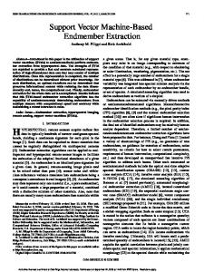
Fig. 1. The uncertainty of the model at some point p (black circle) can be modelled as the realization of a random variable.

gain if we assume that the training time for the Online GP is very small compared to that of the full SVM model. However, this is a reasonable assumption, since the number of training points for the Online GP and hence the number of evaluations of the error surface of the SVM model mainly depends on the dimensionality of the parameter space, which is very small compared to the number of training points for the SVM. There is the remaining question how, given our current Online GP model, we can find the next sample point in parameter space. Here we use the expected improvement criterion as defined by Jones et al. in the EGO algorithm [7]: Formally, the improvement I(p) at some point p in parameter space is defined as I(p) = max(0, Qmin − Y ), where Qmin is our current minimum of the estimated generalization error of the SVM model and Y = N (ˆ µ(p), σ ˆ (p)) (see fig. 1). Note, that µ ˆ(p) is the expected model value at p. Indeed, I is a random variable, because Y is a random variable (it models our uncertainty about µ ˆ(p)). To obtain the expected improvement we simply take the expectation   Qmin − µ ˆ(p) ˆ(p))Φ E[I(p)] = (Qmin − µ (3) σ ˆ (p)   Qmin − σ ˆ (p) +ˆ σ (p)φ σ ˆ (p) where Φ and φ are the standard normal distribution and density function. The expected improvement can be viewed as a function E[I(p)] : P → R and can be evaluated cheaply over the whole parameter space in contrast to the costly evaluations of the error surface of the SVM model (see fig. 2). This is, because we just need the predictions of the ready trained Online GP, which is fast. Now the idea is to sample at that point next, for which the expected improvement becomes maximal, i.e. we

Fig. 2. The expected improvement for an example function. The next sample point would be set where the expected improvement is highest (arrows).

are looking for ˜ = arg max E[I(p)] p p

(4)

This is a global optimization problem for itself, but in contrast to our original problem (1) the solution can be computed cheaply, e.g. by the DIRECT algorithm [12], because of the reasons described above. DIRECT is a sampling algorithm which requires no knowledge of the objective function gradient. Instead, the algorithm samples points in the domain, and uses the information it has obtained to decide where to search next. The DIRECT algorithm will globally converge to the maximal value of the objective function [12]. The name DIRECT comes from the shortening of the phrase “DIviding RECTangles”, which describes the way the algorithm moves towards the optimum. Now we have all ingredients which describe our algorithm to tune SVM and kernel parameters. In the listing 1 we give an overview over the whole procedure, which we call EPSGO (Efficient Parameter Selection via Global Optimization): Beginning from an intial Latin hypercube sampling we train an Online GP, look for the point with the maximal expected improvement, sample there and update our Online GP. Thereby it is not so important that our Online GP really correctly models the error surface of the SVM in parameter space, but that it can give a us information about potentially interesting points in parameter space where we should sample next. We continue with sampling points until some convergence criterion is met. In our case we decided to stop, if the difference between the current best value of Q and the old one is small, and the squared difference between the maximal expected improvement and the average expected improvement is less than 10% of the standard deviation of the expected improvement. These statistics of the expected improvement

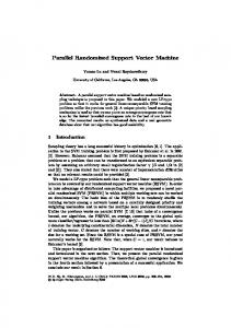
can be computed using Latin hypercube sampling over the whole parameter space (– note again, that these calculations are very fast). The idea is to make sure, that the expected improvement over the whole space is almost equally small. To prevent long searches we also stopped, if Qmin did not change during the last 10 iterations. B. Relationship to Existing Global Optimization Methods The EPSGO algorithm can be viewed as a special variant of the EGO algorithm proposed by Jones et al. [7] for globally optimizing costly target functions. While the EGO algorithm uses a DACE model, which has to be retrained from time to time, we use an Online GP which can be updated efficiently as soon as a new sample point arrives. Jones et al. use a branchand-bound algorithm to maximize the expected improvement, while we take the DIRECT algorithm, which has no nead for the computation of bounds. III. E XPERIMENTS We evaluated our method on 5 classification and 4 regression datasets from the UCI Machine Learning repository1 : the Iris, Glass, Wine, Cleveland Heart and Wisconsin Breast Cancer dataset for classification, and the Boston Housing, Triazines, Pyrimidines and Auto-MPG dataset for regression. Additionally, we included a noisy sinc (sin(x)/x) function (10% normally distributed random noise) in the range -15 to +15 as a standard example for regression and a variant of Wieland’s two spirals with 200 points per class and 3 coils (fig. 3, fig. 4). All data was normalized to mean 0 and 1 http://www.ics.uci.edu/~mlearn/MLSummary.html

Algorithm 1 The EPSGO algorithm Input: function Q to measure gen. error l, u: parameter bounds Output: Qmin , pˆ, # Q-evaluations (neval ) D = dim(P) create N = 10D sample points p1 , ..., pN in [l, u] using Latin hypercube sampl. compute Q(pi ), i = 1, ..., N Qmin = mini Q(pi ) pˆ = arg mini Q(pi ) train Online GP neval = N REPEAT ˜ = arg maxp E[I(p)] (computed by DIRECT) p compute std. dev. and mean of E[I(p)] Qnew = Q(˜ p) if Qnew < Qmin Qmin = Qnew pˆ = p˜ end update Online GP neval = neval + 1 UNTIL convergence

standard deviation 1 before training. On all experiments we chose a RBF kernel with width σ. Additional SVM parameters were C for classification, and C and  for regression tasks, respectively. A one-against-one approach was used to deal with the multiclass case in the classification experiments. As quality measure Q for each set of parameters we used 5-fold cross-validation. We compared our EPSGO method to a grid search with log C ∈ {−2, ..., 14}, log σ ∈ {−5, ..., 7} and (for the regression datasets) log  ∈ {−8, ..., −1} by means of an extra level of 5-fold cross-validation. On the Triazines and Pyrimidines dataset we used the predefined training and testing folds. We also compared our algorithm to the pattern search method of Momma and Bennett with and without bagging (PS/PS-Bag) and a bagged version of EPSGO (EPSGO-Bag). The bagging was performed over 5 models, i.e. we have 5 times the computational effort as without bagging. Table I shows the results of the comparisons of EPSGO to a grid search and the pattern search method without bagging (PS). On the classification data EPSGO needs less than 10% of the search steps of a grid search and leads to almost identical results. On the regression data the advantage becomes even more obvious. Here we need around 1% of the search steps, and in 1 case (noisy sinc function) we obtain a signficicantly better result than with grid search. Thereby significance was tested by means of a paired t-test at 5% signficance level. Compared to the PS method, EPSGO in 7 cases obtains significantly lower error rates, which shows that the pattern search method without bagging often suffers from the problem of local minima and lacks robustness. At the same time on average the number of search steps performed by EPSGO is comparable to those performed by the PS method (table III). The next comparisons are made between the bagged version of the pattern search method (PS-Bag), the EPSGO algorithm and a bagged version of the EPSGO algorithm (EPSGO-Bag) (table II). Obviously PS-Bag neads 5 times the number of search steps of PS. However, this significantly higher amount of computation time only in 4 cases leads to a significant lower error rate of PS-Bag compared to EPSGO. In 6 cases EPSGO is significantly better. The bagged version of EPSGO, EPSGOBag, in 6 cases obtains significant lower error rates, while never being significantly worse than PS-Bag. This again shows the higher robustness and insensitivity to local minima of the EPSGO approach compared to the PS approach. The number of search steps performed by EPSGO-Bag on the regression data on average is slightly higher than those performed by PS-Bag (table III). Compared to EPSGO EPSGO-Bag obtains significantly lower error rates in 3 cases. IV. D ISCUSSION All in all we see that EPSGO/EPSGO-Bag achieve a substantially higher robustness and insensitivity to local minima compared to the PS/PS-Bag. The obvious reason for this is, that the pattern search dependens on the random initialization of just 1 starting point. This dependecy can be reduced by

TABLE I

1.2

5- FOLD CROSS - VALIDATION ERROR ± STANDARD ERROR ON CLASSIFICATION ( FIRST PART OF TABLE ) AND REGRESSION DATA ( SECOND PART ). F OR THE CLASSIFICATION DATA THE MEAN CLASSIFICATION LOSS IN %, FOR THE REGRESSION DATA THE MEAN SQUARED ERROR IS REPORTED . COMPARED TO

S IGNIFICANT IMPROVEMENTS OF EPSGO PS ARE MARKED BY “*”, DETORIATIONS BY “-”.

S IGNIFICANT IMPROVEMENTS OR DETORIATIONS COMPARED TO GRID SEARCH ARE MARKED BY “†” AND “—”. T HE VALUE IN BRACKETS

measured data target

1 0.8 0.6 0.4 0.2

SHOWS THE NUMBER OF SEARCH STEPS NEEDED UNTIL CONVERGENCE . 0

Data

EPSGO

grid search

PS

2 spirals Iris Glass Wine Heart Cancer

0.25 ± 0.3∗ 3.43 ± 1.9∗ 29.15 ± 2.6 1.1 ± 0.7∗ 43.78 ± 2.6 3.08 ± 0.3∗

0.75 ± 0.5 4.74 ± 1.7 31.51 ± 3.3 1.68 ± 1.1 43.42 ± 2.4 3.08 ± 2.7

23.25 ± 9.8 6.87 ± 3.1 29.6 ± 1.8 10.27 ± 6.9 47.15 ± 2.4 7.77 ± 4.1

Sinc ·10−2 Housing ·10−2 Triazines ·10−4 Pyrimidines ·10−2 Auto-MPG ·10−2

14.18 ± 2.3†

37.06 ± 2.1

19.51 ± 5.5

15.35 ± 5.3

13.51 ± 2.2

16.98 ± 2.8

6.95 ± 3.4∗

7.29 ± 3.7

25 ± 16

0.2 ± 0.1∗

0.23 ± 0.2

53.68 ± 13.6

12.49 ± 1.9

19.51 ± 5.5

−0.2 −0.4 −15

−10

−5

Fig. 3.

0

5

10

15

Noisy sinc function.

20 ∗

11.79 ± 1.7

15 10 5

TABLE II C OMPARISON OF EPSGO, EPSGO-BAG AND PS-BAG . 5- FOLD ± STANDARD ERROR ON CLASSIFICATION ( FIRST PART OF TABLE ) AND REGRESSION DATA ( SECOND PART ). S IGNIFICANT IMPROVEMENTS OF EPSGO/EPSGO-BAG COMPARED TO PS-BAG ARE MARKED BY “*”, DETORIATIONS BY “-”. S IGNIFICANT

0 −5

CROSS - VALIDATION ERROR

IMPROVEMENTS OF

EPSGO-BAG COMPARED TO EPSGO ARE MARKED “†”, DETORIATIONS BY “—”.

BY

Data

EPSGO

EPSGO-Bag

PS-Bag

2 spirals Iris Glass Wine Heart Cancer

0.25 ± 0.3∗ 3.43 ± 1.9− 29.15 ± 2.6− 1.1 ± 0.7− 43.78 ± 2.6− 3.08 ± 0.3

1.25 ± 0.7∗ 0 ± 0† 2.75 ± 3† 0±0 2.61 ± 2.6† 3.37 ± 0.6

8.75 ± 2.9 0±0 0±0 0±0 4.29 ± 4.3 3.66 ± 0.7

Sinc ·10−2 Housing ·10−2 Triazines ·10−4 Pyrimidines ·10−2 Auto-MPG ·10−2

14.18 ± 2.3∗

15.15 ± 2.2∗

71.05 ± 21.7

15.35 ± 5.3∗

14.32 ± 3.2∗

28.6 ± 3.8

6.95 ± 3.4∗

6.24 ± 3.6∗

59 ± 13

0.2 ± 0.1∗

0.59 ± 0.4∗

1.5 ± 0.7

∗

11.79 ± 1.7

∗

12.84 ± 1.8

19.09 ± 2.2

−10 −15 −20 −20

−15

Fig. 4.

−10

−5

0

5

10

15

20

Two spirals with 200 points per class.

TABLE III AVERAGE NUMBER OF SEARCH STEPS NEEDED BY THE DIFFERENT METHODS . Method EPSGO PS EPSGO-Bag PS-Bag grid search

Classification 24 ± 4 22 ± 0 120 ± 23 110 ± 0 384

Regression 33 ± 2 32 ± 0 206 ± 33 160 ± 0 3072

using bagging, as proposed by Momma and Bennett, which imposes a much higher computational burden. However, it is still a clearly observable disadvantage compared to our EPSGO method. It is remarkable, that EPSGO without using bagging (and hence being much faster than PS-Bag) in our experiments signficantly outperforms PS-Bag more often than vice versa. For practical purposes it depends on the user’s point of view, whether it is worth taking the higher computational effort of bagging compared to the usual win of lower error rates. If one wants to use bagging, then the EPSGO-Bag method offers a robust way, which at the same time is not very sensitive to local minima, to obtain low error rates while still being very efficient compared to a grid search. Compared to the bagged version of the pattern search EPSGO-Bag on average needs a slightly higher number of search steps. If one does not want to spend the extra time for bagging, then EPSGO without bagging is a good alternative. It leads to results comparable to a grid search, while performing a much faster search in parameter space. This advantage increases, the more parameters we have to tune. V. C ONCLUSION We proposed an efficient method to perform model selection for SVM which is not dependent on special properties of the kernel, e.g. differentiability. Our method is very general and applicable for classification as well as regression tasks. It is a special variant of the EGO algorithm by Jones et al. [7] used in global optimization. We use an Online Gaussian Process to learn a model in parameter space and sample new points, where the expected improvement is maximal. To efficiently find the maximum of the expected improvement we employ the DIRECT algorithm. Comparisions of our method to a usual grid search show the high win of performance with regard to the number of search steps needed. At the same time we obtain error rates which are at least as good. Compared to the pattern search method of Momma and Bennett our approach reveals a better robustness and insensitivity to local minima. This is observable even, if bagging is used in combination with the pattern search. R EFERENCES [1] O. Chapelle and V. Vapnik. Model selection for Support Vector Machines. In S. Solla, T. Leen, and K.-R. Müller, editors, Adv. Neural Inf. Proc. Syst. 12, Cambridge, MA, 2000. MIT Press. [2] O. Chapelle, V. Vapnik, O. Bousqet, and S. Mukherjee. Choosing Multiple Parameters for Support Vector Machines. Machine Learning, 46(1):131 – 159, 2002. [3] V. Cherkassky and Y. Ma. Practical selection of svm parameters and noise estimation for svm regression. Neural Networks, 17(1):113 – 126, 2004. [4] L. Csato and M. Opper. Sparse online gaussian processes. Neural Computation, 14(3):641 – 669, 2002. [5] J. Dennis and V. Torczon. Derivative-free pattern search methods for multidisciplinary design problems. In Proc. 5th AIAA/USAF/NASA/ISSMO Symposium on Multidisciplinary Analysis and Optimization, pages 922 – 932, 1994.

[6] T. Hastie, S. Rosset, R. Tishbirani, and J. Zhu. The entire regularization path for support vector machines. J. Machine Learning Research, 5:1391 – 1415, 2004. [7] D. Jones, M. Schonlau, and W. Welch. Efficient global optimization of expensive black-box functions. J. Global Optimization, 13:455 – 492, 1998. [8] J. Kwok. The evidence framework applied to support vector machines. IEEE Transactions on Neural Networks, 11(5):1162 – 1173, 2000. [9] M. Law and J. Kwok. Bayesian support vector regression. In Proc. 11th Int. Workshop on AI and Statistics (AISTATS 2001), pages 239 – 244, 2001. [10] D. MacKay. Gaussian Processes - A Replacement for Supervised Neural Networks? In Proc. Neural Inf. Proc. Syst., 1997. Lecture note. [11] M. Momma and K. Bennett. A pattern search method for model selection of support vector regression. In SIAM Conf. on Data Mining, 2002. [12] C. Perttunnen, D. Jones, and B. Stuckman. Lipschitzian optimization without the lipschitz constant. J. Optimization Theory and Application, 79(1):157 – 181, 1993. [13] C. Willams. Prediction with gaussian processes: From linear regression to linear prediction and beyond. Technical Report NRG/97/012, Aston University, UK, 1997.