On the parameter optimization of Support Vector ... - Semantic Scholar

Journal of Integrative Bioinformatics, 9(3):201, 2012

http://journal.imbio.de

Paulo Gaspar1 , Jaime Carbonell2 and Jose´ Lu´ıs Oliveira1* 1

´ University of Aveiro, DETI/IEETA. Campus Universitario de Santiago, 3810 - 193 Aveiro, Portugal, http://bioinformatics.ua.pt/ 2

Carnegie Mellon University, Language Technologies Institute. 5000 Forbes Avenue, Pittsburgh, PA 15213, USA Summary Classifying biological data is a common task in the biomedical context. Predicting the class of new, unknown information allows researchers to gain insight and make decisions based on the available data. Also, using classification methods often implies choosing the best parameters to obtain optimal class separation, and the number of parameters might be large in biological datasets. Support Vector Machines provide a well-established and powerful classification method to analyse data and find the minimal-risk separation between different classes. Finding that separation strongly depends on the available feature set and the tuning of hyper-parameters. Techniques for feature selection and SVM parameters optimization are known to improve classification accuracy, and its literature is extensive. In this paper we review the strategies that are used to improve the classification performance of SVMs and perform our own experimentation to study the influence of features and hyper-parameters in the optimization process, using several known kernels.

1 Introduction After their introduction in the world of classifiers, support vector machines (SVM) have been widely studied and applied for their reliable performance in non-probabilistic classification and regression [1, 2, 3]. Multiple applications to real problems have been reported to use SVM based models, such as time series forecasting [4], hand writing recognition [5], text categorization [2], bankruptcy prediction [6], face identification and recognition [7], biological and medical aid [1, 3], among many other fields. In order to classify data, SVMs first find the maximal margin which separates two classes and then outputs the hyperplane separator at the center of the margin. New data is classified by determining on which side of the hyperplane it belongs and hence to which class it should be assigned. However, some input spaces might not be linearly separable, and therefore kernel functions are used to map the input space into a higher-dimensional feature space where the data can be more easily separated. The optimal kernel to use depends on the classification problem and the available data, and it usually has specific parameters than can be controlled to fine-tune the SVM performance. * To

whom correspondence should be addressed. Email: [email protected]

doi:10.2390/biecoll-jib-2012-201

1

Copyright 2012 The Author(s). Published by Journal of Integrative Bioinformatics. This article is licensed under a Creative Commons Attribution-NonCommercial-NoDerivs 3.0 Unported License (http://creativecommons.org/licenses/by-nc-nd/3.0/).

On the parameter optimization of Support Vector Machines for binary classification


However, even when using powerful kernels, sometimes data might not be fully separable, and some tolerance has to be considered when calculating the separating hyperplane. For that, Cortes and Vapnik [8] suggested a soft margin improvement to the original SVM algorithm by introducing slack variables that measure the degree of misclassification for each training instance. A penalty function is added to the problem as a sum of all slack variables, in order to penalize misclassified examples and create a trade-off between generalization and error when looking for the best separation. The penalization of misclassified examples can then be controlled using a weight constant for the penalty function, which is tuned as an SVM parameter (C). The weight can be further extended to a vector form and penalize different training examples at different proportions, but this flexibility can easily lead to creation of over-fit models. Thus, the training of an SVM consists of the following1 minimization problem: minw,ξ { 12 ||w||2 + C

∑

i ξi }

Where w represents the hyperplane normal vector and C is the weight of the penalty function which is formulated by the sum of all ξ slack variables [8].

2 SVM Optimization Given the presence of parameters in the SVM, and possibly in the kernel, that can influence the outcome of the training and classification, it is only natural that these can be fine-tuned to improve its performance. The most basic approach in SVM classification improvement is controlling the slack-variables penalty weight (C) and looking for the best trade-off between allowing misclassification errors and generalizing the model. High values of C will largely penalize misclassified examples, and therefore the resulting hyperplane will be one that strongly avoids classification errors, even when sacrificing generalization. Ultimately, a C = ∞ will lead into a hard-margin SVM behaviour. On the other hand, low values only lightly penalize misclassifications, and the result might be an erroneous separation [9]. Being a parameter of the minimization problem, it is independent of kernel choice, and can always be adjusted. When using kernels other then the linear, they might also have tunable parameters. One of the most common strategies is using a Radial Basis Function (RBF) kernel and optimising its sigma parameter jointly with the C parameter. This method is applied, for instance, by Wu et al [6] to optimize an SVM model capable of predicting bankruptcy. While the RBF kernel is usually used for its flexibility in fitting data, other popular kernels such as the polynomial or sigmoid [10] kernels are also applied and optimized in a similar fashion. For example, in [11], Ali et al have centered attentions in the polynomial kernel and developed methods for the selection of its parameters using classical statistical theory. Besides the kernel and SVM parameters, the data itself plays a crucial role when separating data into two classes, as the SVM bases its algorithm in using the data values to plot each training example in a high dimensional space. The translation to the high dimensional space is of the responsibility of the kernel, but the ease of separation greatly depends on the available feature set. It is well established that features have a large influence on how well data can be separated 1

subject to: ci (w · xi − b) ≥ 1 − ξi , 1 ≤ i ≤ n


2




into two classes, depending largely on the correlation of each feature to its class [12, 13]. Moreover, not all features play a positive role and some might even contribute negatively to the classification process. It becomes important to select the best sub-set of features that improves the ability of the SVM to generalize the model. Thus, many SVM optimization strategies focus on the process of feature selection (FS) [14, 15]. Furthermore, different combinations of these four strategies (selecting the correct kernel, adjusting kernel parameters, adjusting the misclassification penalty, and selecting the best sub-set of features) can lead into significant improvements in classification performance. For instance, in [16], Huang et al provide a study on the joint optimization of C and gamma parameters (using the RBF kernel), and feature selection using Grid search and genetic algorithms. We further extend their approach and compare different kernels and combinations of hyper-parameters, trying to assess the influence and outcome of each approach. Moreover, to optimize the parameters and simultaneously perform feature selection, the parameters can be encoded together with feature selection bits into a single vector, and evolved by an heuristic like simulated annealing. The search algorithm explores the possible permutations and tries to find the best combination of parameters and sub-set of features in an evolutionary fashion [14, 6, 17, 18]. We choose an heuristic and not other strategies (such as gradient descendent, as Chapelle et al propose [19]) for their ease of adding extra parameters to the search, speed of exploration, and no need for further calculations. Nonetheless, besides the extension of literature on the subject of SVM optimization using heuristics like genetic algorithms and distinct kernels, there is still a gap in having a structured comparison of different kernels and selection of parameters under the pressure of optimization. The majority of studies addressing the tuning of hyperparameters (SVM and kernel parameters) often do not consider feature selection, or assess optimization only on a single domain of their research, or perform their optimization using only a single kernel. For instance, one very complete study is that of Huang and Wang [16], where they show that the simultaneous optimization of kernel parameters and feature selection significantly improves classification accuracy of SVMs. Nonetheless, the study is limited to the RBF kernel, and the assessment of performance is achieved using accuracy as a measure, which can lead to a weak form of characterizing classification results when using unbalanced data sets [20]. Another relevant and similar study is that of Sterlin et al, where genetic algorithms are also used to optimize the hyperparameters of an SVM, and four data sets are used to test the hypothesis and compare it to a multi-layer perceptron. Again, only the RBF kernel is used and there is not selection of features. In order to address this gap and assess the best strategies for SVM optimization, in this paper we experiment, analyse and compare several kernels in different parameter combinations under simulated annealing optimization, testing in nine data sets from different domains and with different configurations.

3 Methods In order to optimize the parameters using simulated annealing (SA), the selected parameters are placed in a vector form and that vector is evolved to find the best combination of parameters. The evolution is achieved by modifying a random value in the vector in each iteration of the


3




algorithm, and evaluating the performance of the SVM using the parameters in the new vector. If the new vector achieves a better performance, then it becomes the current vector. However, if not, there is still a probability of accepting the new vector (therefore avoiding local maxima), which depends on its performance and on the current iteration number. As the iterations go by, the probability of accepting worse solutions decreases. The optimization and classification toolboxes from Matlab2 were used to configure and run the SA and SVM. The SA ran for a maximum of 1000 iterations, re-annealing every 300. The parameters to optimize in each experiment were encoded in a vector, bound to maximum and minimum values, and feature selection was represented using a bit string (also in the vector). To evaluate the evolving parameter vector, a fitness function was created which trained and classified the SVM with the selected parameters, using a 10 x 2-fold cross validation with random train and test sets created in each fold. An average f1-score of the classifications is then returned as a performance measure of the parameter vector. We used the matlab integrated version of Suykens least-squares support vector machine [21] to find the separating hyper-plane. We studied 6 different kernels by optimizing their parameters: 1) Linear: k(x, y) = xT y + c, which does not have any parameters to optimize. 2) Polynomial: k(x, y) = (xT y + 1)d , where we optimize the degree d. 3) Radial Basis Function: k(x, y) = exp(− ||x−y|| ), where we optimize the σ value. 2σ 2 2

4) Sigmoid(MLP): k(x, y) = tanh(αxT y+c), where we optimize the α slope and c intercept constant. 5) Cauchy: k(x, y) = (1 +

||x−y||2 −1 ) , σ

where we optimize the σ value.

6) Log: k(x, y) = −log(||x − y||d + c), where we optimize the degree d and constant c. The Linear, Polynomial and Gaussian kernels were selected for their popularity as a common choice, and average good performance. We further extended our experiments to use the Hyperbolic tangent kernel [22] for its resemblance with neural networks, and even being already demonstrated as less preferable than RBF kernels [10] have been found to perform well in practice. We also used the long-tailed Cauchy kernel from Basak [23] and the Log kernel [24]. Though there are studies involving the development and adaptations of new kernels using heuristics [25, 26], we intended to evaluate current literature’s kernels and not to create dataset-specific kernels. Furthermore, the SVM penalty weight C varied between 1 and 1000. The α, σ’s and c (log kernel constant) parameters varied between 1 and 100. The Log kernel and polynomial degrees d varied between 1 and 10. The sigmoid intercept constant varied between -50 and -1.

4 Experiments Several heterogeneous datasets were selected from the UCI machine learning repository [27]. These sets come from different domains such as wine quality (DS1), heart disease (DS2), adult 2

Matlab 7.10.0 (R2010a). All the scripts and data that were used can be downloaded at http://bioinformatics.ua.pt/support/svm/data2.zip


4




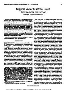
income (DS3), stock data (DS4, not obtained from the UCI), SPECT heart images (DS5), abalone data (DS6), Parkinson’s disease (DS7), Hepatitis (DS8), and Bank Marketing (DS9). The sets were modified to remove incomplete entries, and transform all information into numerical data, and were also prepared for binary classification by selecting examples from only two classes. The datasets were selected in order to obtain a heterogeneous group in that they have different number of examples (entries), different number of features, variate skewness of classes, and different starting baseline results, as shown in Table 1. To build a baseline, the datasets were first classified by a simple SVM using a linear kernel and the default penalty weight (constant C) of 1, with 40 x 2-fold cross validation. The validation was performed by randomly separating the data into two sub-sets (train and test), with each subset containing half of the positive and negative class entries of the original dataset. By creating different train and test sets on each fold, we avoid biasing the average result to the selected sub-sets. The average value of the harmonic mean of precision and recall (f1-measure) of the classifications of each data set was considered for the subsequent optimization experiments (Table 1). Table 1: Datasets used in the experiments. Skew is calculated as the ratio of negative classes.

Data Sets information and base result DS1 DS2 DS3 DS4 DS5 DS6 DS7 DS8 DS9

Source Wine Quality Heart Disease Adult Income Abalone SPECT images Stock data Parkinsons Hepatitis Bank

Set Size 1000 297 1000 2835 267 793 195 129 1521

Nr Features 11 13 12 7 22 27 23 18 17

Skew 77.3% 53.9% 75.5% 53.9% 20.6% 59.8% 24.6% 18.6% 65.8%

Average F1 0.438 0.804 0.494 0.429 0.879 0.646 0.849 0.864 0,709

Std 0.04 0.007 0.035 0.02 0.017 0.031 0.015 0,022 0,009

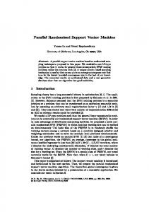
The datasets are also heterogeneous in the types of features that are included, that is, there are features with floating point continuous values, discrete features and binary features. Some features that were originally textual labels were converted into discrete values. 4.1 Optimization Parameters To analyse kernels and their performance on an optimization framework, we created different experiments where we independently test each kernel and fine-tune their parameters. We also include the penalty weight C, and perform different combinations of parameters. Also, since feature selection is often neglected in reports of SVM optimization, we performed different experiments for each kernel where we add/remove feature selection in the optimization. This allows the assessment of the improvement power that feature selection offers. The combinations of selected parameters (SP) are depicted in Table 2. The two parameters for both the sigmoid and log kernels were optimized simultaneously. For each of these combinations, the simulated annealing algorithm is run in each data set, optimizing its parameters to maximize the f1-score obtained by training and testing an SVM. doi:10.2390/biecoll-jib-2012-201

5





SVM Parameters kernel

Selected parameters SP1 SP2 SP3

C FS C

FS

Sigmoid

SP4 SP5

C C

α, c α, c

FS

RBF kernel

SP6 SP7

C C

σ σ

FS

Polynomial kernel

SP8 SP9

C C

poly degree poly degree

FS

Cauchy

SP10 SP11

C C

σ σ

FS

Log

SP12 SP13

C C

degree and c degree and c

FS

Linear kernel

5 Results Each experiment (SP) was performed with simulated annealing optimization, and the best combination of values for the hyper-parameters and features selection was recorded, as well as the performance of the support vector machine using those combinations. The results, which are an average of a 10 x 2-fold cross-validation, were compared with the base results, and the relative improvement of each experiment after optimization is shown in Table 3. The cells are coloured from red to blue (red is worst) to quickly show the overall improvements. Table 3: Results of the experiments on several data sets. For each data set, the F1-measure of each experiment is presented as a relative improvement of the baseline result.

The average value of relative improvements made by each selected parameters experiment in each data set is shown to better compare the several parameter sets. Also, the standard deviation doi:10.2390/biecoll-jib-2012-201

6


Table 2: Used combinations of selected parameters (SPi ). C is the SVM penalty weight; FS stands for feature selection; the σ, α, c, and degree are kernel parameters.


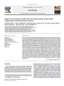
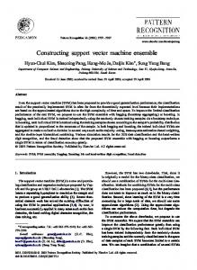
allows assessing the dispersion of the improvement over the data sets. When clustering Table 3 by experiment, one can visualize a bars chart where the effects of each optimization are observed (depicted in Figure 1). Since some f-measure results were below the baseline result (meaning that they performed worst than the non-optimized linear kernel), there are negative improvements, mainly on the sigmoid kernel.

Figure 1: Each selected parameter set (SP) is presented along with its results for each data set (DS). The vertical axis represents the relative improvement in F-score in relation to the baseline value.

Moreover, to assess the statistical significance of the results, the baseline F-scores were compared with the final F-scores using a two-tailed paired t-test. The p-values are shown in Table 4. Since not all values are below the α significance level of 5%, some of the experiments do not reject the null hypothesis. This means that the improvement was not statistically significant for those kernels. The linear, RBF and polynomial kernels stand out for presenting sound improvement. Table 4: The p-values were calculated using a two-tailed t-test.

6 Discussion Optimization of SVMs using search algorithms is a common procedure to obtain better classification results. By optimizing the hyper-parameters we can perceive the generalization power of each kernel, which otherwise might not show using random or default parameters. However, authors refer different strategies, using several kernels and approaches to tune the SVM performance. Overall, in our experiments, we obtained an average 11% relative improvement to the simple SVM classification, and if we only consider the kernels which had valid statistical significance, the average improvement increases to almost 20%. Also, using a heterogeneous group of datasets from different domains allowed us to assess how kernels behaved on average. The extension of 9 datasets and the different combinations of parameters clearly shows the superiority of some kernels over others even when not considering a specific domain.


7




When analysing results we can see several details regarding each experiment. For instance, when optimizing the selection of which features are used in the SVM (feature selection, SP2) in the simplest kernel, the different results for each dataset do not vary much. In fact, they had the smallest standard deviation, which is less than half of the second smallest standard deviation (SP13 with 16% std), while still attaining almost 11% average improvement. This, alone, proves the usefulness and power of performing feature selection, while not depending much on the dataset. Also important to note is that, in experiments where FS was added to the parameter set (SP3, SP5, SP7, SP9, SP11 and SP13), the average result always increased (3% on average) and the standard deviation remained unchanged. Thus, feature selection successfully improves SVM classification while maintaining generalization. On the other hand, when optimizing the misclassification penalty alone in a linear kernel (SP1), the results show a much larger deviation than feature selection, but also better results. Here, the standard deviation might be less important since the misclassification penalty translates the ease of class separation, which is very dependent on the dataset. Adding feature selection to C (SP3) diminishes this effect and further improves classification. When looking at the standard deviation in an overall fashion, we see a high average value for both experiments (17%) and datasets (12%). This suggests that the choice of best strategy for optimization strongly depends on the dataset. However, it might also reflect a trade-off between improvement and generalization, such that the more a model is optimized to improve f-score the higher it is over-fit. This is perceived in the large correlation3 that exists (0.95) between the average values and their corresponding standard deviations in the experiments that had statistical significance. Also, a strong negative correlation (-0.81) was found between the averages of each dataset and the corresponding initial baseline values, translating that sets with lower base results tend to be significantly more improved than higher base results. This becomes useful to assess how much an optimization would improve the classification of an arbitrary dataset: if an SVM base result is low, the optimization tends on yielding larger improvements. Though several studies [26, 28, 29] have mentioned that there is no single best kernel which has best performance in all problem domains, we have experimentally assessed the superiority of some kernels over others in a very heterogeneous group of datasets. Namely, the multilayer perceptron kernel (sigmoid) has shown to return very poor classification performance on the majority of the datasets. Also, both Log and Cauchy kernels had a bad overall performance and were almost always below other more popular kernels like the RBF, polynomial, or linear kernels and even the base result. Nonetheless, recalling the no free lunch theorem [30], the Log kernel achieved the best result of all experiments in the Hepatitis dataset (DS8), and the Sigmoid kernel was also above average in this same dataset. When evaluating the experiments kernel-wise, the RBF kernel stands-out with the larger average improvement (22%) closely followed by the polynomial kernel (21%) and the linear kernel (16%). However, the RBF also shows the largest variation (23% std) while the polynomial kernel has less disperse improvements (18% std) over the datasets, making it more attractive considering the small difference in average improvement. When dealing with the skewness of datasets, the optimization results of the first and third experiments (SP1 and SP3) show a considerable amount of positive linear dependence (72% cor3

All correlations were calculated as person correlations.


8




relation) with the ratio of negative classes. Datasets with large amounts of negative examples (in comparison to the positive ones) have smaller base results (-0.84 correlation), which in turn, as explained before, tend on yielding larger improvements. Acting on the input space makes the linear kernel more sensitive to skewness, and controlling the weight of the penalty function aids in separating the classes. On the other hand, the sigmoid kernel (in SP5) shows no correlation with class skewness, but since the results are not statistically significant this might not be a considerable effect.

7 Conclusions The most common techniques in literature for the optimization of the classification performance of SVMs are tackling the misclassification penalty and kernel parameters, often by fine-tuning them together. We have created a performance optimization test-bench using 9 heterogeneous datasets and 6 different kernels, while selecting different combinations of parameters to finetune. In our experiments we verified the potential of performing feature selection to improve the classification abilities in a stead fashion (we saw a low variance between datasets) while combining it with the hyper-parameters, which is often ignored in literature. We also verified a high standard deviation in the overall experiments, suggesting that the optimal optimization approach greatly depends on the characteristics of the dataset, such as its size, number of features, and class skewness. Nonetheless, the most common kernels in literature obtained the best improvements (RBF, Polynomial and Linear), while other known kernels achieved surprisingly poor results, even below the basic approach of using a linear kernel without any optimization. We also found a positive tendency that datasets with low base results have in greatly being improved by optimization. This means that when dealing with SVMs yielding weak classification performance, it is generally the case that optimization will be able to strongly enhance those results.

References [1] I. Guyon, J. Weston, S. Barnhill, and V. Vapnik. Gene selection for cancer classification using support vector machines. Machine Learning, 46(1):389–422, 2002. [2] G. Siolas et al. Support vector machines based on a semantic kernel for text categorization. In IJCNN, volume 5, pages 205–209. Published by the IEEE Computer Society, 2000. [3] M.F. Akay. Support vector machines combined with feature selection for breast cancer diagnosis. Expert Systems with Applications, 36(2):3240–3247, 2009. [4] L. Cao. Support vector machines experts for time series forecasting. Neurocomputing, 51:321–339, 2003. [5] C. Bahlmann, B. Haasdonk, and H. Burkhardt. Online handwriting recognition with support vector machines-a kernel approach. In Proceedings of the Eighth International Workshop on Frontiers in Handwriting Recognition, 2002., pages 49–54. IEEE, 2002.


9




[6] C.H. Wu, G.H. Tzeng, Y.J. Goo, and W.C. Fang. A real-valued genetic algorithm to optimize the parameters of support vector machine for predicting bankruptcy. Expert Systems with Applications, 32(2):397–408, 2007. [7] G. Guo, S.Z. Li, and K. Chan. Face recognition by support vector machines. In Automatic Face and Gesture Recognition, 2000. Proceedings. Fourth IEEE International Conference on, pages 196–201. IEEE, 2000. [8] C. Cortes and V. Vapnik. Support-vector networks. Machine Learning, 20(3):273–297, 1995. [9] T. Joachims. Learning to classify text using support vector machines: Methods, theory, and algorithms. Computational Linguistics, 29(4):656–664, 2002. [10] H.T. Lin and C.J. Lin. A study on sigmoid kernels for SVM and the training of nonPSD kernels by SMO-type methods. Technical report, Department of Computer Science, National Taiwan University, URL http://www.csie.ntu.edu.tw/ cjlin/papers/tanh.pdf 2003. [11] S. Ali and K.A. Smith. Automatic parameter selection for polynomial kernel. In IEEE International Conference on Information Reuse and Integration, 2003. IRI 2003, pages 243–249. IEEE, 2003. [12] L. Yu and H. Liu. Feature selection for high-dimensional data: A fast correlation-based filter solution. In Proceedings of the Twentieth International Conference on Machine Learning (ICML-2003), Washington DC, 2003, volume 20, pages 856–863, 2003. [13] M.A. Hall. Correlation-based feature selection for machine learning. PhD thesis, Citeseer, 1999. [14] F. Holger and O. Chapelle. Feature selection for support vector machines by means of genetic algorithms. In Proceeding of the 15th IEEE International Conference on Tools with Artificial Intelligence (ICTAI’03), pages 142–148, 2003. [15] Y.W. Chen and C.J. Lin. Combining SVMs with Various Feature Selection Strategies. In Isabelle Guyon, Masoud Nikravesh, Steve Gunn, and Lotfi Zadeh, editors, Feature Extraction, volume 207 of Studies in Fuzziness and Soft Computing, pages 315–324. Springer Berlin / Heidelberg, 2006. [16] C.L. Huang and C.J. Wang. A GA-based feature selection and parameters optimization for support vector machines. Expert Systems with Applications, 31(2):231–240, 2006. [17] F. Friedrichs and C. Igel. Evolutionary tuning of multiple SVM parameters. Neurocomputing, 64:107–117, 2005. [18] M. Liepert. Topological Fields Chunking for German with SVMs: Optimizing SVMparameters with GAs. In Proceedings of the International Conference on Recent Advances in Natural Language Processing (RANLP), Bulgaria. Citeseer, 2003. [19] O. Chapelle, V. Vapnik, O. Bousquet, and S. Mukherjee. Choosing multiple parameters for support vector machines. Machine Learning, 46(1):131–159, 2002.


10





[21] J.A.K. Suykens and J. Vandewalle. Least squares support vector machine classifiers. Neural Processing Letters, 9(3):293–300, 1999. [22] M. Sellathurai and S. Haykin. The separability theory of hyperbolic tangent kernels and support vector machines for pattern classification. In IEEE International Conference on Acoustics, Speech, and Signal Processing, 1999, ICASSP’99, volume 2, pages 1021–1024. IEEE, 1999. [23] J. Basak. A least square kernel machine with box constraints. In 19th International Conference on Pattern Recognition, 2008, ICPR 2008, pages 1–4. IEEE, 2008. [24] S. Boughorbel, J.P. Tarel, and N. Boujemaa. Conditionally positive definite kernels for svm based image recognition. In IEEE International Conference on Multimedia and Expo, 2005, ICME 2005, pages 113–116. IEEE, 2005. [25] T. Howley and M.G. Madden. The genetic kernel support vector machine: Description and evaluation. Artificial Intelligence Review, 24(3):379–395, 2005. [26] A. Zien, G. Rätsch, S. Mika, B. Schölkopf, T. Lengauer, and K.R. Müller. Engineering support vector machine kernels that recognize translation initiation sites. Bioinformatics, 16(9):799–807, 2000. [27] UCI machine learning repository. http://archive.ics.uci.edu/ml/. [28] B. Schölkopf and A.J. Smola. Learning with kernels: Support vector machines, regularization, optimization, and beyond. The MIT Press, 2002. [29] A. Ali and A. Abraham. An empirical comparison of kernel selection for support vector machines. In Proceedings of the second international conference on hybrid intelligent systems: design, management and applications. The Netherlands: IOS Press, pages 321– 30, 2002. [30] D.H. Wolpert and W.G. Macready. No free lunch theorems for optimization. IEEE Transactions on Evolutionary Computation, 1(1):67–82, 1997.


11


[20] R. Akbani, S. Kwek, and N. Japkowicz. Applying support vector machines to imbalanced datasets. Machine Learning: ECML 2004, pages 39–50, 2004.

On the parameter optimization of Support Vector ... - Semantic Scholar

On the parameter optimization of Support Vector ... - Semantic Scholar

Suggest Documents

Feature Selection and Parameter Optimization of Support Vector ...

Efficient Parameter Selection for Support Vector ... - Semantic Scholar

A Heuristic for Free Parameter Optimization with Support Vector

Optimization of Experimental Model Parameter ... - Semantic Scholar

parameter optimization of deterministic dynamic ... - Semantic Scholar

Parameter optimization of advanced machining ... - Semantic Scholar

COMPARISON OF SUPPORT VECTOR MACHINE ... - Semantic Scholar

Parameter selection for support vector machines

Twin Support Vector Machines Based on the ... - Semantic Scholar

Parameter Optimization and Field Validation of the ... - Semantic Scholar

Parameter Optimization for the Extraction of ... - Semantic Scholar

Combining Support Vector Regression with ... - Semantic Scholar

Support Vector Machine-Based Endmember ... - Semantic Scholar

Parallel Randomized Support Vector Machine - Semantic Scholar

Pattern Classification Using Support Vector ... - Semantic Scholar

Parallel Support Vector Machines - Semantic Scholar

Support vector machine classification and ... - Semantic Scholar

Marketing segmentation using support vector ... - Semantic Scholar

Recurrent Support Vector Machines - Semantic Scholar

Recurrent Support Vector Machines - Semantic Scholar

Pattern Recognition General support vector ... - Semantic Scholar

Constructing support vector machine ensemble - Semantic Scholar

Relevance Feedback using Support Vector ... - Semantic Scholar

KNOWLEDGE-BASED SUPPORT VECTOR ... - Semantic Scholar