this approach directly depends on the size of the components' local state space ... techniques synergistically combine into efficient symbolic verification, as ... We consider systems comprised of many copies of a few basic building blocks. .... An alternative technique makes use of the following ... loops, subroutine calls, etc.
Efficient Reduction Techniques for Systems with Many Components E. Allen Emerson and Thomas Wahl Department of Computer Sciences and Computer Engineering Research Center The University of Texas, Austin/TX 78712, USA
Abstract. We present an improved approach to verifying systems involving many copies of a few kinds of components. Replication of this type occurs frequently in practice and is regarded a major source of state explosion during temporal logic model checking. Our solution makes use of symmetry reduction through counter abstraction. The efficiency of this approach directly depends on the size of the components’ local state space, which is exponential in the number of local variables. We show how program analysis can significantly reduce the local state space and can help towards a succinct BDD representation of the system. Our reduction techniques synergistically combine into efficient symbolic verification, as documented by promising experimental results.
1
Introduction
We consider systems comprised of many copies of a few basic building blocks. Examples include collections of concurrent processes executing the same program, but also compositions of distinct kinds of homogeneous subsystems, such as the readers-writers protocol. Systems of this type are a primary source of state explosion during temporal logic model checking, characterized by the potential to incur a state graph much larger than the description of the system. In this paper, we show how program analysis techniques can significantly enhance the benefit of symmetry reduction to limit this problem. A system is symmetric with respect to a group of bijections on the state space if the transition relation R is invariant under each bijection π, i.e. if R equals {(π(s), π(t)) : (s, t) ∈ R}. The bijections amount to permutations of the processes. States that are identical up to such permutations are considered equivalent. The quotient structure that is derived naturally from this equivalence is bisimilar to the original structure. Of particular interest is the case of full symmetry. Here, the above condition on R is satisfied for every permutation π. Such symmetries allow up to an exponential reduction in structure size. Also, they occur frequently in practice, especially in connection with systems of replicated homogeneous process components. This work was supported in part by NSF grants CCR-009-8141 and CCR-020-5483, and SRC contract 2002-TJ-1026. Email: {emerson|wahl}@cs.utexas.edu
Model checking on the quotient structure requires an efficient way of determining whether two states are equivalent. This so-called orbit problem turned out to be the bottleneck of symmetry reduction, particularly for symbolic representation using binary decision diagrams. The BDD that contains pairs of symmetry-equivalent states is provably of intractable size and must therefore be avoided [CEFJ96]. One solution that applies to the case of fully symmetric systems is counter abstraction [Lub84,GS92]. It is based on the observation that two global states, viewed as vectors of local states of processes, are equivalent under arbitrary permutations exactly if for every local state L, the number of occurrences of L is the same in the two states. For example, the three states (A, A, B), (A, B, A) and (B, A, A) are equivalent under full symmetry, since in all of them, two of the processes reside in local state A, one in B. The states can be represented succinctly as the tuple (2A, 1B) of counters. The approach not only avoids the orbit problem, but also reduces a system of size ln (n processes, each with l possible local states) to one of size roughly nl (l counters, each with range [0..n]). With respect to the number of processes, the system size has been reduced from exponential to polynomial [ET99,EW03]. Unfortunately, the local state explosion problem, encountered often in practice, can have a negative impact on these benefits. A local state of a process is a valuation of the process’ local variables. For example, each of the 2m assignments of values to m boolean local variables forms a local state. The size of the local state space is thus exponential in the number of local variables. Introducing a counter for every local state becomes infeasible in connection with symbolic data structures like BDDs, which require bits to be reserved a priori for each counter. One objective of this paper is to limit local state explosion. We show that an analysis of the input program describing the processes’ behavior often reveals opportunities to reduce the number of local states that actually must be monitored. Although in principal a local state is defined by the values of all local variables, it is sufficient to restrict attention to those that are live at certain points in the program, i.e. whose current value is used along some future path. Experience shows that for many programs, only a fraction of their variables are live at any time during execution. We go on to demonstrate instances of static local reachability analysis that can further cut down on the size of the abstract system: The counter of an unreachable local state is invariably 0 and does therefore not have to be introduced into the counter-abstracted model. Many cases of unreachable local states can be detected through an over-approximation of the local state space of each process or by statically analyzing the process’ program, before building the global Kripke model. Live variable analysis is frequently applied in compiler optimization to improve run time performance. A key contribution of this paper is to show a way in which it can be very beneficial for verification as well, namely through a potentially exponential reduction of the size of the counter-abstracted model. In the best case, if no two of m boolean local variables are ever live together, the
abstract model needs only 2 counters per program control point, despite 2m conceivable local states. The techniques can be applied algorithmically. They are efficient, since they operate on the source code, which is usually small compared to a Kripke model. Finally, the proposed reductions are exact, i.e. the reduced system has the same behavior as the original one (they are bisimilar). Languages intended for modeling asynchronous systems often allow changing the local state of many components in one atomic step. For example, a reset operation might cause every component to return to its initial state. In the abstract program, this requires a synchronous update of a large number of counter variables. We show how serialization can greatly reduce the complexity of symbolically representing such statements, which seem to occur quite frequently in practice. The serialized execution is efficient and preserves all properties of the system expressible in the temporal logic CTL. Our framework allows symbolic model checking of arbitrary CTL formulas for systems specified in the high-level and flexible modeling language of the Murϕ verifier [MD]. We exploit symmetry using counter abstraction whenever possible. (Sub-) Systems with full symmetry, as marked by Murϕ’s scalarset type, are converted into a hybrid representation of counters (replacing the symmetric part) and specific state variables. We structure this paper as follows. Section 2 introduces the model of computation, and provides some background. Section 3 presents the techniques to reduce the local state space. Section 4 describes the serialization of expensive atomic actions. We conclude with experimental results, comparison to related work and future prospects.
2
Preliminaries
Model of Computation. We assume a system of concurrent process components with an interleaving model of computation. Replicated processes are instantiations of a program template. Any number of templates is allowed; each gives rise to a fully symmetric subsystem. Each process has its own local variables, declared in its template. All variables and statements declared outside any template are referred to as global. We thus permit compositions of distinct fully symmetric subsystems, which allows us to model systems like Readers-Writers (two symmetric clusters) or microprocessors with separate symmetries in channels, memory addresses, registers, etc. Symmetry Reduction. Intuitively, the Kripke model M = (S, R) of a system is symmetric if it is invariant under certain transformations π of its state space S. In our case of process symmetry, π takes over the task of permuting the processes. Formally, if li denotes the local state of process i, i ∈ [1..n], π is derived from a permutation on [1..n] and acts on a state s as π(s) = π(l1 , . . . , ln ) = (lπ(1) , . . . , lπ(n) ). Given π, we derive a mapping at the transition relation level by defining π(R) = {(π(s), π(t)) : (s, t) ∈ R}. Structure M is said to be fully symmetric if π(R) = R for all π.
The relation θ := {(s, t) : ∃π : π(s) = t} on S defines an equivalence between states, known as orbit relation; the equivalence classes it entails are called ¯ = (S, ¯ R), ¯ where S¯ is a chosen set of orbits. It induces a quotient structure M ¯ representatives of the orbits, and R is defined as ¯ = {(¯ R s, t¯) ∈ S¯ × S¯ : ∃s, t ∈ S : (s, s¯) ∈ θ ∧ (t, t¯) ∈ θ ∧ (s, t) ∈ R}.
(1)
¯ is up to exponentially In case of full symmetry, i.e. given π(R) = R for all π, M smaller than M and bisimulation equivalent to M ; the bisimulation relation is ¯ ∩ θ. Relation ξ is actually a function and maps state s to the unique ξ = (S × S) representative s¯ of its equivalence class under θ. Properties of systems of concurrent components are usually expressed using indexed atomic propositions, such as Ci , stating that in the given state process i ¯ , the (maximal) satisfies some property C. To perform model checking on M propositional subformulas of the property in question must be invariant under permutations. A permutation acts upon a propositional formula by permuting the indices of the atomic propositions appearing in it. Invariance then means propositional equivalence. For example, the propositional formula C1 ∨ . . . ∨ Cn is invariant under any permutation action. Summarizing, for two states (s, s¯) ∈ ξ and any formula f over propositional subformulas p such that p ≡ π(p) is a tautology for every π ∈ G, M, s |= f
⇔
¯ , s¯ |= f. M
(2)
Counter Abstraction. For BDD-based symbolic verification, symmetry reduction using the orbit relation is likely to be space-inefficient, as shown in detail by Clarke et. al. [CEFJ96]. An alternative technique makes use of the following observation in order to represent orbits. Two states, i.e. vectors of local state identifiers, are equivalent under θ (identical up to permutation) exactly if for every local state L, the frequency of occurrence of L is the same in the two states—permutations only change the order of elements, not their values. An orbit can therefore be represented as a vector of counters, one for each local state, that records how many of the processes are in the corresponding local state. For example, in a system with local states N , T and C, the states (N, N, T, C), (N, C, T, N ), and (T, N, N, C) are all symmetry-equivalent; their orbit (which contains other states as well) can be represented compactly as (2N, 1T, 1C), or just (2, 1, 1). In practice, it is often possible to rewrite the program describing a fully symmetric system such that its variables are local state counters in the first place (before building a Kripke structure). This procedure is known as counter abstraction, on which this paper concentrates. The advantage of the counter notation is clear: the symmetry is implicit in the representation; the very act of rewriting the program from the specific notation of local state variables into the generic [ET99] notation of local state counters implements symmetry reduction. Subsequently, model checking can be applied to the structure derived from the counter-based program without further considerations of symmetry.
Input Language. We adopted the input language of the Murϕ explicit state verifier, because it is widely known, has been used to verify non-trivial examples, and already has a built-in datatype to mark full symmetry. The complete language specification is available from [MD]. In brief, transitions in Murϕ are known as rules, which may have a guard that must be satisfied for the rule to be enabled, i.e. able to fire. Firing means executing the rule’s body, leading to a new state. The body consists of assignments and high-level statements like loops, subroutine calls, etc. Our verifier accepts a program in this language and performs symbolic model checking with respect to CTL specifications (unlike the Murϕ tool, which analyzes the reachable state space for invariant violations using an explicit representation of states). Symmetry is marked in the Murϕ input language using the scalarset datatype, a symmetric subrange of the integers. Syntactic restrictions guarantee full symmetry of the resulting state graph.1 For example, a system of n pairwise interchangeable processes can be declared as var proc: array[scalarset(n)] of basetype, where basetype is some user-defined data type that represents local variables. Our verifier recognizes this type of symmetry and ultimately translates the program into an equivalent one, with the specific processes proc[0..n-1] replaced by counters.
3
Local State Space Reduction
High-level modeling languages allow users to specify the behavior of processes in terms of (assignments to) global and local variables. The concept of local states is implicit and must first be extracted from the program. This is, at least in theory, straightforward. A local state is given by a valuation of the local variables. Quantitatively, let m be the number of local variables declared in a program template, and let V1 , . . . , Vm be the ranges of those variables. It follows that there are |V1 | × . . . × |Vm | possible local states of each process. If we naively introduce one counter per local state in order to perform counter abstraction, we obtain a number of counters that is exponential in m and hence in the input program size. The number of local states is an important factor for the efficiency of counter abstraction. With BDD-based symbolic model checking, bits need to be explicitly allocated for every counter, whether it is relevant for program execution or not. It is therefore crucial for the performance of counter abstraction to detect situations in which keeping a counter to monitor a local state is unnecessary. Such a situation might arise because some variable values in a local state are unused in the program and hence do not matter (section 3.1), or because the local state is known to be unreachable (section 3.2). 1
Compliance with the restrictions is not entirely verified by the compiler, see [MD].
3.1
Live Variable Analysis
We assume the program executed by the processes is specified as sequential code with individual control points that demarcate atomic actions. In this case, the local state space of a process contains a program counter, indicating the statement to be executed next. An analysis of the program allows us to estimate the way data are manipulated. We can exploit this information by only keeping track of values of variables that can possibly be used in the future. Definition 1 (e.g. [Muc97]) A variable x is called live at a control point if there exists a path to a future moment2 at which the value of x is used, and x is not assigned along the path. Otherwise, x is dead at the control point. Consider the following example. Each of n processes has two local boolean variables, nonempty and locked , and a program counter PC ∈ [0..7]. There is a global variable q ∈ [0..n], which counts waiting processes. Process i’s program is shown in figure 1.
0. nonempty i := (q > 0); q := q + 1 1. if nonempty i then 2. locked i := true 3. wait until ¬locked i { execute restricted code here } 4. if q = 1 then 5. q := 0; goto 0 6. some j : PC j = 3 : locked j := false 7. q := q − 1; goto 0
lock process i wait for other process to unlock i access to some resource, etc.
unlock some proc. j waiting at line 3
Fig. 1. Program text for process i
Variable nonempty is live only at program line 1. It is used only there, and it is not live before reaching 1, since it is assigned right before in line 0. The consequence is that we do not have to remember the value of nonempty at any program line other than 1. For instance, the two local states (4, false, false) and (4, true, false), written in the order (PC , nonempty, locked ), do not have to be distinguished, since they differ only in the value of the dead (in line 4) variable nonempty. Notice that both local states are otherwise legitimate and in fact reachable. A similar argument holds for variable locked . It turns out to be live only at line 3, and thus needs to be remembered only at that point of the program. How much does this analysis help counter abstraction? The straightforward approach introduces a separate counter for each conceivable local state, of which there are |[0..7]| × |{false, true}|2 = 32. In contrast, following the above analysis, at all lines except 1 and 3, no local variable other than the PC matters. For 2
“Future” is meant to include the present, i.e. the current program line.
line 1, we only record the value of nonempty, and for line 3, only locked . The table below lists the local states that the program needs to monitor, using again the notation (PC , nonempty, locked ) with ’−’ for irrelevant values: (0, − , − ) (2, − , − ) (4, − , − ) (7, − , − ) (1, false, − ) (3, − , false) (5, − , − ) (1, true , − ) (3, − , true ) (6, − , − ) We have thus reduced the number of local states to keep track of from 32 to 10. The formal justification for not recording dead variables is as follows. Assume each process has a program counter PC and m other local variables v 1 , . . . , v m . The concurrent execution of the program P by the processes in an interleaved fashion defines a Kripke structure M = (S, R). Recall that a global state s ∈ S is given by a valuation of all global variables, and by assigning a local state to each process. Definition 2 Consider the binary relation ∼ on the local state space of each process, defined as (PC x , x1 , . . . , xm ) ∼ (PC y , y 1 , . . . , y m ) if 1. PC x = PC y , and 2. xi = y i for each i ∈ [1..m] such that variable v i is live at line PC x . Relation ∼ can be extended to a relation ≈ on the global state space S by defining s ≈ t if s and t agree on all global variables and for each process p, the local states lp (s) and lp (t) of p in s and t, respectively, satisfy lp (s) ∼ lp (t). Theorem 3 Relation ≈ is an equivalence relation on S. Moreover, the quotient ¯ of M with respect to ≈ is bisimilar to M with the canonical bisimstructure M ulation relation B := {(s, [s]) : s ∈ S} relating a state to its equivalence class under ≈. Proof : For the first part, we start by showing that ∼ is an equivalence relation on the local state space. Reflexivity and symmetry of ∼ follow immediately from properties of equality. For transitivity, (PC x , x1 , . . . , xm ) ∼ (PC y , y 1 , . . . , y m ) and (PC y , y 1 , . . . , y m ) ∼ (PC z , z 1 , . . . , z m ) implies PC x = PC z . Assume an i such that variable v i is live at PC x . From the equivalence of the first two states, we conclude xi = y i , and from the last two, we conclude y i = z i , thus xi = z i . Regarding ≈, since both “agreement on all global variables” and ∼ are equivalence relations, so is ≈. ¯ = (S, ¯ R) ¯ is defined as S¯ = {[s] : s ∈ S} For the second part, the quotient M ¯ = {(¯ (set of equivalence classes of ≈), and R s, t¯) ∈ S¯ × S¯ : ∃s ∈ s¯, t ∈ t¯ : (s, t) ∈ R}. Given s ∈ S and s¯ = [s], we have to show two things: 1. Assume t such that (s, t) ∈ R. Then let t¯ = [t]. t and t¯ are related under B. ¯ it follows that (¯ ¯ By definition of R, s, t¯) ∈ R. ¯ Then, by definition of R, ¯ there exist s′ ∈ s¯, 2. Assume t¯ such that (¯ s, t¯) ∈ R. ′ ′ ′ t ∈ t¯ such that (s , t ) ∈ R. By the semantics of interleaved execution, this means that s′ , t′ agree on the local states of all processes except one, say p,
which possibly changes its local state from lp (s′ ) to lp (t′ ). Since s, s′ ∈ s¯, they have the same PC value, they agree on all global variables, and further on all local variables of process p (in fact, of all processes) except possibly some dead variables, whose values, by definition, are not used at the current PC . It follows that executing P from local state s gives the same result t′ as executing P from s′ , hence (s, t′ ) ∈ R. We can therefore choose t := t′ and have t ∈ t¯ and (s, t) ∈ R. � ¯ can be implemented fully auCounter abstraction of the reduced structure M ¯ tomatically, and without first building M , as follows. Determining live variables is a data flow analysis problem. A variety of solutions exist, of a complexity that is in practice usually low-degree polynomial in the size of the input program; see for example [Muc97]. The result is, for each value of the program counter, a list of the variables that are live just before the corresponding line. Stepping through the program, we create a counter variable for each partial valuation of the local variables of the form (PC , x1 , . . . , xk ) such that xi is a value of local variable v i , and v i is live at the given PC . Dead variables are not expanded into possible local states. 3.2
Local Reachability Analysis
Suppose L is a local state (i.e. a valuation of local variables) that is not reachable by any process. In the counter-abstracted program, the corresponding counter nL is invariably zero. If the unreachability of L is known a priori, we do not have to introduce nL as a variable in the abstract program, and the translation into counters does not have to consider L. Formally, we define the local reachability problem as follows. Given a local state L and a system of concurrent processes, determine whether there is a reachable global state in which some process is in local state L. In general, this problem is of course a model checking problem by itself. However, in order to perform counter abstraction, we do not need to know the exact set of reachable local states; any over-approximation suffices. In fact, not performing such an analysis at all is tantamount to using all (conceivable) local states in creating counters. The better we approximate the precise set of reachable local states, the fewer counters we have to introduce, resulting in increased efficiency. The set of reachable local states can be approximated in several ways. One solution is to build a Kripke model of the given program template, instantiated with only a single process, say process 1. Guards that express dependencies on local states or local variables of other processes are treated conservatively, i.e. they are replaced by true if under an even number of negations (they have positive polarity), and by false otherwise. For example, the guard ∃i : Ai is replaced by A1 ∨ true and hence by true, whereas ∀i : Bi is replaced by B1 ∧ true and hence by B1 . Guards on global variables are likewise replaced by true or false, depending on their polarity. Assignments to global variables are discarded. Essentially, local information of other processes and global variables are viewed as part of an unpredictable environment. The result is a Kripke structure that
over-approximates the behavior of a process. Since this local structure can be expected to be exponentially smaller than the global structure of the concurrent composition of the processes, standard reachability analysis can be performed on it. Every local state reachable in the global structure is also reachable in the local structure. Another technique to approximate reachable local states is borrowed from compilers, which sometimes optimize program behavior by confining the number of values that a local variable can have at some program point. Local states not satisfying these limits are unreachable. Examples for such techniques are constant propagation, constant folding, copy propagation, integer interval arithmetic and perhaps even alias analysis (depending on the expressive power of the programming language).3 Consider the following contrived program, which prints an input number a in some numerical base and the character with ASCII code a, denoted by chr (a). 0. 1. 2. 3. 4.
const minprint := 32 base := 16 read a if minprint ≤ a < minprint + 96 then print convert (a, base), ": ", chr (a)
least printable ASCII code choose a numerical base if a among 96 printable characters
Variables minprint and base degenerate to constants, since there is only one (dynamic) assignment to them. After replacing every occurrence by 32 or 16, resp. (constant propagation), these variables do not participate in the construction of local states. More interestingly, in line 4 we know after constant folding that a satisfies 32 ≤ a < 128, so local states with PC = 4 and a < 32 or a ≥ 128 are unreachable. Assuming base ∈ {2, 8, 10, 16} (binary, octal, etc.) and a ∈ [0..255], the conceivable state space of the above program with local variables PC , base and a has size 5 · 4 · 256 = 5120. Using the above observations and the fact that a is live only at lines 3 and 4, we obtain a number of counters that need to be introduced of only 1 + 1 + 1 + 256 + 96 = 355 (one term for each program line). More generally, regarding the potential of these observations, note that if we have shown for only a single local variable that it cannot assume a particular value at some program line, the total number of local states is reduced by at least 2m−1 , given m local variables. (However, for several variables at the same program line, the respective sets of local states eliminated may not be disjoint.) Discussion. Both analyses presented in section 3 are performed efficiently on the source code of the program. As described here, both techniques are static, i.e. they do not require (partial) execution of the program and ignore communication between components. Instead, they exploit modularity. This makes them a fast front-end to counter abstraction. Another point to note is that live variable analysis (section 3.1) requires an input model with highly predictable flow of control, such as a sequential program, as opposed to, say, a set of rules among 3
See for instance [Muc97] for a taxonomy and precise definitions of these techniques.
which the next is non-deterministically chosen. In contrast, local reachability analysis via the local Kripke structure (section 3.2) is fit for any input model. The overall benefit of counter abstraction is dependent on the ratio between the number of local states l and the number of participating processes n. Since the counter-abstracted system can be shown to have size O(nl ), as compared to O(ln ) for the original system, the case n ≫ l promises most benefits. If l ≫ n, then at any time during execution most counters are zero. For space-efficiency, an explicit-state model checker may use a compressed notation for all zero-valued counters. Symbolically, zero-suppressed BDDs [Min01] may be applicable, but this technique does not capture the benefits of live variable analysis, where the counters shown to be irrelevant are non-zero. Moreover, since the set of zerovalued counters varies over time, counters for all local states must still be declared initially. The advantage of the techniques in this section is that they reduce the number of counters before even building a symbolic model; irrelevant ones are simply not present.
4
Serializing Synchronization Constructs
In modeling languages intended for describing asynchronous systems, the granularity of interleaving is determined by whatever the programmer puts inside an atomic action. Such languages therefore usually support constructs that change the local state of several processes at the same time. Common examples are broadcasts to all processes in a symmetric subsystem instructing them to reset their local state in order to recover from a deadlock, or to invalidate their cache data. We call such statements synchronization constructs. We show that the straightforward way to implement them abstractly using counters can lead to complex BDDs, and describe an alternative that allows for a more efficient solution. 4.1
Straightforward Counter Abstraction
In this section, we denote the value of local variable x in local state L by x(L) (“x in L”). Assume, for the purpose of an example, every process has a local boolean variable x, and consider the statement (before counter abstraction) for i : xi := false.
(3)
It changes the local state of all processes i where currently xi = true. The straightforward translation of this simple statement into one based on counters is rather involved. For all local states L with x(L) = true, counter nL must be set to zero (no process with x = true exists after the execution of (3)). Further, for local states L with x(L) = false, let L′ := L x=true denote the local state identical to L except that x(L′ ) = true. Counter nL increases by nL′ , since all processes in L′ transit to L. These two steps can be implemented by executing for L : x(L) = true : do nL := 0 for L : x(L) = false : do nL := nL + nL′ with L′ := L x=true
(4) (5)
in parallel, or sequentially in the order (5), (4). Parameter L in statement (5) ranges over almost all possible local states, namely all where x is fixed to be false. In the worst case, the number of choices for L is thus exponential in the number of local variables other than x. For all such choices of L, the counter addition operation in (5) must be modeled symbolically. Even after the reductions described in the previous section, there is an evident potential for blow-up in the representation of statement (5) as a BDD. Things get worse if variable x has a range Vx of cardinality greater than 2. The choice of the “source state” L′ in (5) (which processes leave in order to enter L) is then not uniquely determined any more. In general, for each L, there are |Vx | − 1 possibilities for L′ . The intuition for this complexity is an artifact of counter abstraction. In an assignment like for i : xi := false, the current value of xi is overwritten and therefore normally not of further interest. With counter abstraction, however, we need to know this value since the counter for the future local state increases by the value of the counter for the current local state (L vs. L′ in (5)). The solution to avoid the complexity is to disentangle steps (4) and (5) so as to execute the original statement (3) in a serial fashion. The key is that this can be done in a way that preserves all properties of the program. 4.2
Enforcing Serialized Execution
Compound statements of the form for i : stmti are often such that the result does not depend on the order in which the individual stmti are executed. This is guaranteed, for example, if i ranges over the process indices of a fully symmetric (sub)system. To implement for i : stmti serially, execution switches to a mode of operation in which the only enabled statement is stmti ; we call it the serial mode. It will be turned off again once every process has executed stmti —the order is irrelevant. To see how such a mode can be enforced, we first turn our attention to a subclass of statements. In the following, we view a statement as a mapping from states to states in the form stmt: S → S. Definition 4 A statement stmt is called idempotent if stmt2 = stmt, i.e. executing it twice has the same effect on any state as executing it once. Observation 5 Statement stmt is idempotent exactly if, and only if, for all states s, stmt(s) ∈ p for stmt’s fixpoint predicate p = {s ∈ S : stmt(s) = s}. Thus, executing an idempotent stmt produces a state satisfying p, and every state satisfying p is unchanged by stmt. All assignments x := expr such that x does not appear in expr are idempotent; the fixpoint predicate is x = expr . For conditional statements if cond then x := expr , the fixpoint predicate is (¬cond ) ∨ (x = expr ). Consider now a statement for i : stmti with idempotent stmti , and let pi be stmti ’s fixpoint predicate. For an intermediate state s during serial mode, the question whether some process j still needs to execute stmtj can be resolved using pj : the answer is yes exactly if pj is false at s. The serial mode must therefore be maintained as long as not all pi are true. More precisely,
1. let b be a fresh global boolean variable, initial value false 2. the statement for i : stmti is replaced by b := ∃i : ¬pi 3. the guard of every existing statement in the program (including the new one in number 2) is strengthened by the conjunct ¬b 4. the following guarded statement is added to the program, for any process j: b ∧ ¬pj −→ { stmtj ; b := ∃i : ¬pi }
This translation procedure is applied to all for statements with an idempotent body. One new bit is introduced for each such for statement, resulting in a vector ~b of new variables. The old and the new program give rise to Kripke structures M and M ′ , respectively. Property equivalence of M and M ′ . Let B denote the disjunction of all bits in ~b; this evaluates to true over a global state in M ′ exactly if M ′ is currently executing one of M ’s for statements. First we observe that M ′ is neither an over- nor an under-approximation of M , since some behavior was removed from M , other behavior was added. It turns out, however, that all properties written in the temporal logic CTL4 are preserved if we ignore states of M ′ in serial mode in the evaluation of CTL formulas: Theorem 6 Let f be a CTL formula, s a state of M , and let s′ be the unique state of M ′ that satisfies ~b = (false, . . . , false) and is identical to s on all other variables (~b does not occur in s). Then M, s |= f
exactly if
M ′ , s′ |= f ′ ,
where f ′ is recursively defined according to the structure of f : f f f f f f f
atomic proposition: = ¬g : =g∨h: = AF g : = AG g : = A (g U h) : = AX g :
f′ f′ f′ f′ f′ f′ f′
=f = ¬(g ′ ) = g ′ ∨ h′ = AF (g ′ ∧ ¬B) = AG (g ′ ∨ B) = A ((g ′ ∨ B) U (h′ ∧ ¬B)) = AX A (B U (g ′ ∧ ¬B)).
An analogous result holds for formulas with existential path quantifiers. The proof is accomplished by induction on the structure of f and is omitted here. As an example, a safety formula of the form AG good , to be evaluated over M , is translated into AG (good ∨ B) over M ′ , the liveness property AG (req ⇒ AF grant) becomes AG ((req ⇒ AF (grant ∧ ¬B)) ∨ B). 4
For a full description of this logic, see for example [EC82].
One can see that almost all basic modalities are adjusted for verification in M ′ only by adding a propositional disjunct or conjunct (B). Intuitively, the disjunct B allows invariants to ignore states of M ′ in serial mode, whereas the conjunct ¬B requires eventualities to in fact become true in states of M ′ that have a counterpart in M , not in serial mode. A more complex translation is required for the AX modality (last equation in theorem 6). This is no surprise, as the serialization of the for statements does not preserve next-time: a single transition is replaced by a path of length n + 1, for the number n of processes.5 Efficiency. The translated program has no transitions that require all processes to execute an idempotent statement simultaneously. Transitions executed by one process at a time require simple counter increments and decrements by 1, with very efficient BDD implementations. The state space of the new program has as many additional bits as there are idempotent for statements in the original program. The new statement b := ∃i : ¬pi is translated into the abstract statement b := ∃c : c > 0, where c ranges over counters for local states satisfying ¬p. This statement can be expressed very efficiently with a BDD of size logarithmic in the number of counter variables. The additional guard ¬b increases the BDD size of an individual transition by no more than O(1) node. (The bit representing b should precede the bits for the processes’ local states in the BDD variable ordering.) Since some transitions in M are replaced by paths of length n + 1 in M ′ , a fixpoint computation in M ′ may require about n additional iterations. Our experiments show that this overhead is more than compensated by the gain in efficiency due to the reduced BDD complexity of the transition relation. Generalization. The above translation relies on the idempotency condition. A general, and less memory-efficient, solution that handles arbitrary for loops over all processes can be obtained by introducing a fresh bit b local to every process. These bits are initially false; when the for statement needs to be executed, they are set to true. Interestingly, setting all bits to true again requires a for loop over all processes. However, this loop has an idempotent body (bi := true), so the technique presented above can be applied. Then, an arbitrary process is selected whose bit bi is true (= “waiting for execution”), its individual statement is executed, and bi is set to false. An equivalence result similar to theorem 6 can be formulated.
5
This path is unique up to reordering of execution by the processes. Thus, “AX A” in the last equation of theorem 6 can be equivalently replaced by “AX E”.
5
Experimental Results
In this section we show quantitative results of applying our techniques. Symbolic computations are done with our own model checker UTOOL, which uses the CUDD BDD package [Som]. It takes a program in the input language of the Murϕ explicit-state model checker and performs symbolic verification on it, exploiting symmetry using counter abstraction whenever possible. Our tool is flexible in that it has support for less-than-full symmetries as well. In tables, “Number of BDD nodes” refers to the peak number of BDD nodes allocated at any time during execution. It represents the memory bottleneck of the verification run. In columns titled “Time”, the symbols “s”, “m” and “h” stand for seconds, minutes, and hours, respectively. For comparative explicitstate model checking, we used the Murϕ verifier as available on the Internet (see [MD]). All experiments were run on an i686/1400 Mhz PC with 256MB main memory. The purpose of the first, introductory, example, is to demonstrate the potential of counter abstraction compared to other reduction methods that utilize symmetry (even without applying our program analysis techniques). We consider the classical scenario of r readers and w writers that compete for access to some data. The problem consists of two fully symmetric subsystems, but the global system is asymmetric (due to the writers’ priority). The first algorithm shown in table 1, “Multiple Representatives”, refers to applying symmetry reduction to the Kripke structure derived from the original program, without counter abstraction. This technique allows symmetry equivalence classes (orbits) to be represented by several states. The advantage to an approach using unique orbit representatives is that a state of the orbit can be mapped to that representative for which this mapping is most efficient; see [CEFJ96] for details.6 The next double column lists the results of applying the Murϕ verifier to the counterabstracted program, i.e. non-symbolically. The third algorithm combines counter abstraction and symbolic representation. We see from the table that counter abstraction is—even in its non-symbolic form—more successful than the symbolic multiple representatives approach, which suffers from symmetry reduction overhead. It should be noted that this overhead largely stems from the computation of the a priori representative mapping, which does not make use of the simplicity of the transition relation of this problem. As the results on the right show, counter abstraction was most effective when combined with BDD-based symbolic model checking. The readers-writers scenario is characterized by a small number of local states. In such simple cases, techniques based on local state counters can be successful without techniques as those described in this paper. The second example demonstrates the local state space reduction based on live variable analysis from section 3. In many synchronization algorithms, processes 6
The naive approach using the orbit relation mentioned in section 2 is not exhibited here since it fails already for very small problem instances.
Choice of r, w r
w
8 8 10 10 16 16 30 30 100 100 1000 1000
Symbolic Murϕ: Non-symbolic Symbolic Multiple Representatives Counter Abstraction Counter Abstraction Number of Number of Number of Time Time Time BDD nodes rules fired BDD nodes 19,853 1.4s 11,835 0.6s 1,082 0.0s 41,333 5.8s 25,784 0.6s 1,082 0.0s 223,770 108.0s 140,471 0.7s 1,379 0.1s 2,494,219 1:29m 1,482,854 2.2s 1,379 0.1s — — 159,625,349 162.4s 1,973 0.2s — — — — 2,864 1.5s Table 1. Results for the Readers-Writers problem
denied access to some restricted resource wait (“spin”), constantly polling some global variable. According to [MS91], this can cause performance bottlenecks, and is partially avoidable. We investigated one of the algorithms proposed in [MS91] (the list-based spin-lock without atomic compare-and-swap operation), verifying that no two processes can acquire the resource at the same time, that there is no deadlock in the system, and that processes will eventually gain access to the resource, once requested. The program executed by the processes is similar to that in figure 1 in section 3.1. Symbolic Counter Abstraction . . . without Reductions with Local State Reduction Number Number of Number of Time Time of proc. BDD nodes BDD nodes 5 16,583 1.4s 3,022 0.1s 10 71,224 28.8s 9,366 0.6s 15 156,421 110.4s 17,070 1.5s 30 785,411 25:53m 68,332 19.4s 50 2,643,540 3:34h 207,370 145.9s 70 5,586,017 12:16h 454,360 10:18m Table 2. Results for the MCS Spin Lock algorithm
The table teaches an important lesson. Counters corresponding to local states that have no bearing on the program behavior should be explicitly excluded from the BDD model. The fact that some conceivable local states differ only by irrelevant (dead) variables is not taken care of automatically. The final example illustrates the effect of serializing complex synchronous instructions when working with BDDs. A communication bridge transports data between two ports, performing operations on them in the middle [Sim99]. Processes read the data from the output port. When the output port is full, and no
process is ready to consume the data, the system is in a deadlock-like situation. It recovers from it by instructing all processes to interrupt and be ready to unburden the output port. The message is broadcast to all processes, rather than just sent to one, since the output port would likely be full again quickly if only one data item was read from it. We verified that no data is overwritten at the ports, and that the ports are cleared within a fixed number of steps. The latter property is important for performance guarantees when the bridge is part of a system that is embedded in other devices. The subsystem formed by the processes is, for the purpose of verifying these properties, fully symmetric. Table 3 shows the results for the straightforward counter abstraction of the processes (“simultaneous broadcast”), and for counter abstraction with serialized execution of the broadcast statement. Symbolic Counter Abstraction . . . with simultaneous broadcast with serialized broadcast Number Size of Number of Size of Number of Time Time of proc. trans. rel. BDD nodes trans. rel. BDD nodes 4 10,914 49,576 2.2s 4,177 21,699 2.1s 8 15,850 188,690 10.4s 5,190 66,864 7.7s 16 20,786 830,610 127.4s 6,203 209,157 55.3s 32 25,722 2,683,800 26:43m 7,216 586,938 8:30m 64 30,658 7,310,979 3:36h 8,229 1,955,509 1:12h Table 3. Results for Communication Bridge example
The figures in the table first tell us that the size of the transition relation was reduced by a factor that grows with the size of the problem. This translates into a reduction of the total number of BDD nodes, to the extent of about the same factor. It is also worth noting that the time savings achieved are slightly less than the space savings. One possible reason was hinted at earlier: The serialization requires more iterations during fixpoint computations to converge.
6
Conclusion
We have shown how to integrate program analysis techniques into symmetry reduction based on counter abstraction for exact and efficient model checking, using symbolic representation with BDDs. Our method is most powerful when the given system contains (multiple kinds of) identical components. Our approach appears to be unique in its improvement of counter abstraction using program analysis. Recently, [FBG03], [WS02] and [Yor00] suggest static analysis techniques to optimize BDDs in a concrete (rather than counter abstracted) scenario. The potential savings come from choosing dummy values for dead variables, or from non-deterministic assignments to them. This might
reduce the size of the BDD graph, but does not diminish the number of allocated BDD variables. In contrast, we observe that dead local variables typically result in many redundant (equivalent) local states. All but one of them can be eliminated, significantly reducing the number of counters. This is guaranteed to decrease the number of BDD variables and the size of the BDD graph. In [BR00], the use of compiler optimization techniques similar to ours is suggested to reduce the number of BDD variables to represent reachable states, with different BDDs for different program points. In contrast, the goal of our work is to build a symbolic representation of the overall program, to enable symbolic model checking. This is possible since counter abstraction (which is of no concern in [BR00]) allows us to incorporate live variable information into the abstract state representation, by creating local state counters judiciously. An interesting goal for the future is to apply our methods to a conservative abstraction of an infinite-state system, using truncated counters. An approach to doing this with Murϕ was presented in [ID99]. It is orthogonal to the techniques presented here, since truncation reduces the range of counters, but not their number. Another further direction is to investigate to what extent counters can be used to reduce systems with less than full symmetry, such as rotational symmetry found in the Dining Philosophers example. Our tool currently falls back on other symmetry reduction techniques in such cases. Applying counter abstraction only to fully symmetric systems is still a huge win, since (1) full symmetry is the most frequent symmetry type, (2) it offers greater potential for savings than other symmetries, and (3) other symmetries suffer to a lesser extent from the orbit relation complexity. Acknowledgments. We would like to thank the reviewers for their helpful comments regarding the readability of this paper.
References [BR00]
Thomas Ball and Sriram K. Rajamani. Bebop: A symbolic model checker for boolean programs. In Model Checking of Software (SPIN), 2000. [CEFJ96] Edmund M. Clarke, Reinhard Enders, Thomas Filkorn, and Somesh Jha. Exploiting symmetry in temporal logic model checking. Formal Methods in System Design (FMSD), 1996. [EC82] E. Allen Emerson and Edmund M. Clarke. Using branching time temporal logic to synthesize synchronization skeletons. Science of Computer Programming (SOCP), 1982. [ES90] E. Allen Emerson and Jai Srinivasan. A decidable temporal logic to reason about many processes. In Principles of Distributed Computing (PODC), 1990. [ES96] E. Allen Emerson and A. Prasad Sistla. Symmetry and model checking. Formal Methods in System Design (FMSD), 1996. [ET99] E. Allen Emerson and Richard J. Trefler. From asymmetry to full symmetry: New techniques for symmetry reduction in model checking. In Conference on Correct Hardware Design and Verification Methods (CHARME), 1999.
[EW03]
E. Allen Emerson and Thomas Wahl. On combining symmetry reduction and symbolic representation for efficient model checking. In Conference on Correct Hardware Design and Verification Methods (CHARME), 2003. [FBG03] Jean-Claude Fernandez, Marius Bozga, and Lucian Ghirvu. State space reduction based on live variables analysis. Science of Computer Programming (SOCP), 2003. [GS92] Steven M. German and A. Prasad Sistla. Reasoning about systems with many processes. Journal of the ACM, 1992. [ID96] C. Norris Ip and David L. Dill. Better verification through symmetry. Formal Methods in System Design (FMSD), 1996. [ID99] C. Norris Ip and David L. Dill. Verifying systems with replicated components in Murϕ. Formal Methods in System Design (FMSD), 1999. [Lub84] Boris D. Lubachevsky. An approach to automating the verification of compact parallel coordination programs. Acta Informatica, 1984. [MD] Ralph Melton and David L. Dill. Murϕ Annotated Reference Manual, rel. 3.1. http://verify.stanford.edu/dill/murphi.html. [Min01] Shin-ichi Minato. Zero-suppressed bdds and their applications. Software Tools for Technology Transfer (STTT), 2001. [MS91] John M. Mellor-Crummey and Michael L. Scott. Algorithms for scalable synchronization on shared-memory multiprocessors. Transactions on Computer Systems (TOCS), 1991. [Muc97] Steven S. Muchnick. Advanced Compiler Design & Implementation. Morgan Kaufmann Publishers, 1997. [PD95] Fong Pong and Michel Dubois. A new approach for the verification of cache coherence protocols. IEEE Transactions on Parallel and Distributed Systems (TOPDS), 1995. [Sim99] David E. Simon. An Embedded Software Primer. Addison-Wesley, 1999. [Som] Fabio Somenzi. The CU Decision Diagram Package, release 2.3.1. University of Colorado at Boulder, http://vlsi.colorado.edu/~fabio/CUDD/. [WS02] Farn Wang and Karsten Schmidt. Symmetric symbolic safety-analysis of concurrent software with pointer data structures. In Formal Techniques for Networked and Distributed Systems (FORTE), 2002. [Yor00] Karen Yorav. Exploiting Syntactic Structure for Automatic Verification. PhD thesis, Technion Israel, http://www.cs.technion.ac.il/users/orna/KarenThesis.ps.gz, 2000.