Efficient Selection of Inputs for Artificial Neural Network Models Fernando, T.M.K.G., H.R. Maier, G.C. Dandy and R. May Centre for Applied Modelling in Water Engineering (CAMWE), School of Civil and Environmental Engineering, The University of Adelaide, Adelaide, Australia, E-Mail:
[email protected] Keywords: Artificial neural networks; input identification; mutual information; outliers; robust statistics variable is significant or not. The original algorithm proposed by Sharma (2000) used the bootstrap method with 100 bootstraps to obtain the 95th percentile confidence limit for the PMI. However, as pointed out by Chernick (1999), about 5,000 bootstraps are needed for simple problems and about 10,000 bootstraps for more complicated problems in order to estimate the required confidence intervals reliably. Use of such a large number of bootstraps as the stopping criterion for the PMI algorithm would decrease the computational efficiency of the algorithm significantly, probably to the point of impracticality for most realistic problems.
EXTENDED ABSTRACT The selection of an appropriate subset of variables from a set of measured potential input variables for inclusion as inputs to model the system under investigation is a vital step in model development. This is particularly important in data driven techniques, such as artificial neural networks (ANNs) and fuzzy systems, as the performance of the final model is heavily dependent on the input variables used to develop the model. Selection of the best set of input variables is essential to being able to model the system under consideration reliably. When the available data set is high dimensional, it is necessary to select a subset of the potential input variables to reduce the number of free parameters in the model in order to obtain good generalization with finite data. The correct choice of model inputs is also important for improving computational efficiency. However, the topic of input selection is a difficult one. Real systems are generally complex and mostly associated with nonlinear processes. Consequently, the dependencies between output and input variables, as well as conditional dependencies between variables, are difficult to measure.
The focus of this study is to introduce an alternative stopping criterion for PMI algorithm implementation, which is both robust and computationally efficient. As part of the proposed method, significant PMI scores are treated as outliers in the computed PMI scores. A robust outlier detection technique, the Hampel identifier (Davies and Gather, 1993), is used to evaluate the significance of selected candidate inputs. The reliability of the new technique is first investigated using two nonlinear data series where dependencies of attributes were known a priori. The new technique consistently selects the correct inputs, while being computationally efficient.
Mutual information (MI) has been used successfully to measure the dependence between output and input variables. In contrast to the linear correlation coefficient, which often forms the basis of empirical input variable selection approaches, mutual information is capable of measuring dependencies based on both linear and nonlinear relationships, making it well suited for use with complex nonlinear systems. Partial mutual information (PMI) has been proposed in recent years as a means of measuring conditional dependencies between output and input variables (Sharma, 2000). It is a robust technique for selecting input variables for multivariate, nonlinear, complex natural systems, such as hydrological processes. The PMI approach is a stepwise input variable selection algorithm. Consequently, it is necessary to have a reliable technique to indicate whether a selected candidate
The modified PMI algorithm is then applied to select inputs to forecast salinity in the River Murray at Murray Bridge, South Australia, which are used to develop an ANN model. The results obtained in this study are compared with those obtained in three previous studies which developed ANN models for the same case study. The proposed PMI algorithm identifies only 11 inputs as significant from 1323 candidate inputs. The resulting ANN model has the smallest number of inputs when compared with the models developed in previous studies for this case study, with no loss in predictive performance.
1806
1.
where fx(xi), fy(yi) and fx,y(xi, yi) are the respective univariate and joint densities estimated at the sample data point (Sharma, 2000). This simplifies the integral in (1) to a summation and can be used to obtain kernel density based mutual information efficiently. The Gaussian kernel function (Scott, 1992), together with the Gaussian reference bandwidth (Scott, 1992, Silverman, 1986), are adopted in this study to estimate MI using (2).
INTRODUCTION
In recent years, there has been a significant amount of research on measuring the dependence between two random variables. In contrast, there has been very little work on multivariate or conditional measures of dependence among sets of random variables. The coefficient of linear correlation is the most widely used measure for computing dependence between bivariate data, whereas the partial linear correlation coefficient can be used to measure the conditional dependence between sets of variables. Autocorrelation is widely used to determine the number of lagged variables in modeling time series data. A shortcoming of all of the above measures is that they are based on covariance and therefore only account for linear dependence. However, most real world systems are governed by complex, nonlinear processes and as a result, the dependencies between variables are nonlinear. Mutual information possesses properties that make it well suited to measuring statistical dependence for both linear and nonlinear data. 1.1.
1.3.
The MI criterion can be used to identify dependence between bivariate data. However, as is the case with the linear correlation coefficient, it cannot be used to compute the dependence for multivariate data. To avoid this problem, Sharma (2000) proposed a new stepwise input selection algorithm, the partial mutual information (PMI). PMI provides a measure of the conditional dependence between a new candidate input and already selected inputs and the output. The PMI between the output y and the input x, for a set of already selected inputs z, is given by ⎡ f ' ' ( x' , y' ) ⎤ x ,y ⎥dx'dy' I' = ∫∫ f x ' , y ' ( x' , y' ) loge ⎢ ' ' ⎢⎣ f x' ( x ) f y ' ( y ) ⎥⎦
Mutual Information
For a set of N bivariate measurements, zi = (xi, yi), i = 1,...,N which are assumed to be independent, identically distributed realizations of a random variable Z = (X,Y), with joint probability density fx,y(x,y), mutual information is defined as
I ( X , Y ) = ∫∫ dxdyf x , y ( x, y ) log
Partial Mutual Information
f x , y ( x, y )
(3)
where
x ' = x − E [x | z ] ;
y ' = y − E[y | z ]
(4)
[]
where E ⋅ denotes the expectation operation. The '
'
variables x and y only contain the residual information in variables x and y after considering the effect of the already selected inputs z .
(1)
f x ( x) f y ( y )
where fx(x) and fy(y) are the marginal probability density functions of X and Y, respectively and fx,y(x,y) is the joint probability density function of X and Y.
The discrete version of (3) can be used to approximate the sample PMI and is given as:
1.2.
I' =
Estimation of Mutual Information
Calculation of mutual information is not always easy, as it requires estimation of the marginal probability density functions (pdfs) of x and y and estimation of the joint pdf of x and y. The most widely used approach for estimating MI is based on histograms. However, this approach can be unreliable, which has resulted in the use of kernel based MI estimators (Moon et al., 1995).
1 N
N
∑ log i =1
e
⎡ f x, y ( xi , y i ) ⎤ ⎢ ⎥ ⎢⎣ f x ( x i ) f y ( y i ) ⎥⎦
⎡ f x' , y' ( x ' i , y ' i ) ⎤ ⎢ ⎥ log ∑ e ' ' ⎢⎣ f x ' ( x i ) f y ' ( y i ) ⎥⎦ i =1 N
'
where x i
(5)
'
and y i are the ith residuals in the
sample data set of size N and '
f x ' ( x ' i ), f y ' ( y ' i )
'
and f x ' , y ' ( x i , y i ) are the respective marginal and joint probability densities. In this study, the general regression neural network (Specht, 1991) is used to estimate the conditional expectations in (4), as they are nonlinear and only require estimation of a single parameter. This is in agreement with the approach taken by Bowden et al. (2005).
When using kernel based methods, the mutual information score in (1) can be approximated as
I≈
1 N
(2)
1807
Implementation of the PMI algorithm requires a criterion to decide when to stop the addition of new candidate inputs to the already selected inputs. Sharma (2000) suggested the 95th percentile confidence limit of the sample PMI for this purpose. Sharma’s original algorithm used the bootstrap method with 100 bootstraps to obtain the 95th percentile confidence limit. However, as pointed out by Chernick (1999), approximately 5,000 bootstraps are needed for simple problems and about 10,000 bootstraps for more complicated problems in order to estimate the required confidence intervals reliably. Use of such a large number of bootstraps as the stopping criterion for the PMI algorithm would decrease the computational efficiency of the algorithm significantly, probably to the point of impracticality for most realistic problems. Consequently, the focus of this study is on the development of a reliable and efficient alternative technique to the bootstrap method. 2.
(MAD), respectively. The Hampel distance, or modified Z score (MAD), for a data set {xi } is defined as: Hampel distance= (xi – x0.50 ) / S
(6)
where x0.50 = median and S is the MAD scale estimate defined as (Pearson, 2001) S=1.4826 median {| xi – x0.50 |}
(7)
The factor 1.4826 was chosen so that the expected value of S is equal to the standard deviation σ for normally distributed data. 2.1.
Modified PMI Algorithm
The basic steps in the modified PMI input selection algorithm are as follows: 1. Identify the set of potential inputs that could be useful in modelling the system under investigation. Denote this input set as zin. Denote the vector that will store the selected inputs as z.
PROPOSED METHOD
2. Estimate the PMI between the output and each of the potential new inputs in zin, conditional on the pre-existing input set z by using Equation (5).
The proposed approach is to treat significant PMI scores as outliers in the computed PMI scores. If the highest PMI score is found to be an outlier among the computed PMI scores for a particular step, then the input corresponding to the highest PMI score is a significant input. The rationale behind this approach is that if there are no outliers in the PMI scores, then all PMI scores would have the same level of significance (or in this case, no significance). This would only occur after all significant variables have been selected. Consequently, the presence of outliers indicates the presence of significant PMI scores. It should be noted that this approach does not work if the candidate inputs do not contain non-significant inputs. However, this scenario is unlikely to occur in practice, particularly when dealing with time series applications, where a number of lagged values are considered.
3. Calculate the Hampel distance corresponding to the highest PMI score in step 2. 4. If the Hampel distance for the highest PMI value > 3, add the input variable corresponding to the highest PMI score to selected input set z and remove it from zin. If the highest PMI is not an outlier, go to step 6. 5. Repeat steps 2 – 4 as many times as needed. 6. This step will be reached only when all significant inputs have been selected. 3.
APPLICATION TO DATA SETS WITH KNOWN ATTRIBUTES
Two data sets with known dependence attributes were used to evaluate the reliability of the modified PMI algorithm. The two data series were the nonlinear threshold autoregressive models used by Sharma (2000), including:
As part of the proposed approach, the presence of outliers in the PMI scores is detected using a robust outlier detection technique, the Hampel identifier (Davies and Gather, 1993). This is an improved, robust version of the commonly used “3σ edit rule” or “Z score” approach to outlier detection. For a normally distributed data set, the probability that Z score > 3 is only about 0.3% and is used to detect the outliers in the data set. However, this rule fails in the presence of multiple outliers due to an effect called “masking”. The Hampel identifier replaces the outlier sensitive mean and standard deviation estimates with the outlier resistant median and median absolute deviation from the median
TAR1 – Threshold Autoregressive order 1 ⎧− 0.9 xt −3 + 0.1et xt = ⎨ ⎩ 0.4 xt −3 + 0.1et
if xt −3 ≤ 0 if xt −3 > 0
(8)
TAR2 – Threshold Autoregressive order 2 ⎧− 0.5xt −6 + 0.5xt −10 + 0.1et if xt −6 ≤ 0 xt = ⎨ 0.8xt −10 + 0.1et if xt −6 > 0 ⎩
1808
(9)
where et was Gaussian random noise with zero mean and unit standard deviation for both models. One thousand and forty data points were generated for each of the models. The first 25 points were discarded and the first 15 lags were chosen as potential inputs. In addition to the modified Z score (MAD), the 95th percentile randomised sample PMI was also computed with 1000 bootstraps. The results obtained using the modified PMI algorithm applied to these data sets are shown in Table 1. It can be seen that the modified Z score (MAD) was able to correctly identify the inputs for both nonlinear threshold data sets. In addition, computation of the modified Z score (MAD) was also relatively computationally efficient. In contrast, even with 1000 bootstrap iterations, the 95th percentile randomized sample PMI did not correctly identify the inputs for the TAR2 model. The results obtained indicate that use of the modified Z score (MAD) shows promise as an efficient alternative stopping criterion for PMI algorithm implementation.
Maier and Dandy (1996) considered a total of 16 variables, including daily salinity, flow and river level data at different locations in the lower Murray River (Table 2) for the period 01-12-1986 to 30-06-1992 as potential model inputs. The same data set was used in this study to select model inputs using the modified PMI algorithm. In addition, more recent data for the period 01-071992 to 01-04-1998 were used to verify the real time forecasting capabilities of the developed model. This second validation data set was same as that used by Bowden et al. (2002, 2005). Table 2. Available data and selected maximum lag for each variables Location Murray Bridge Mannum Morgan Waikerie Loxton Lock 1 Lower Overland Corner Downstream of Lock 7 Murray Bridge Mannum Lock 1 Lower Lock 1 Upper Morgan Waikerie Overland Corner Loxton
Table 1. PMI input selection algorithm results for TAR1 and TAR2
Z Score (MAD)
Model
TAR1
Xt-3
0.0662
0.0336
12.6
Xt-13
0.0318
0.0331
0.9
Xt-10
0.5104
0.0301
64.0
Xt-6
0.0718
0.0335
22.5
X t-14
0.0330
0.0324
1.7
TAR2
4.
PMI
95th percentile randomised sample PMI
Selected input
5.
Data type
Abbreviation
Maximum lag (days)
Salinity Salinity Salinity Salinity Salinity Flow Flow
MBS MAS MOS WAS LOS L1LF OCF
74 81 104 102 102 116 100
Flow
L7F
103
Level Level Level Level Level Level Level Level
MBL MAL L1LL L1UL MOL WAL OCL LOL
21 18 116 15 99 69 101 102
INPUT VARIABLE SELECTION
The data set for the period 01-12-1986 to 30-061992 was used to obtain the input variables for the ANN model. Maier and Dandy (1996) used a priori knowledge of the system to select the initial time lags for each variable, whereas Bowden at al. (2005) used the first 60 lags of each variable as potential inputs. Fraser and Swinney (1986) proposed that the time lag corresponding to the first minimum of mutual information should be a better choice for the maximum time lag considered. This MI based criterion has since been used in various hydrological studies (e.g. Phoon et al., 2002). A slightly modified version of the same approach was used in this study to obtain the maximum number of lagged variables to consider as potential inputs. The MI between salinity at Murray Bridge with a 14 day lead time and each variable with different lags was computed and the optimal lag for each variable was selected, depending on the occurrence of first
CASE STUDY
The case study used to further test the effectiveness of the modified PMI algorithm was the forecasting of salinity in the River Murray at Murray Bridge, South Australia, with a lead time of 14 days. Maier and Dandy (1996) have previously developed ANN models for this case study. Bowden et al. (2002, 2005) further investigated different aspects of ANN model development using the same case study and tested the performance of the ANN models in a realtime forecasting simulation on an independent data set. Hence the River Murray salinity data provided a good benchmark for testing the performance of the modified PMI algorithm.
1809
minimum in MI values. The selected potential lags for each variable are given in Table 2. This results in total of 1323 potential initial inputs with 2023 samples.
values, were scaled to lie in the range -0.8 to 0.8. The number of nodes in the hidden layer affects the performance of the trained network and therefore should be optimised. In general, networks with fewer hidden nodes are preferable, as they usually have better generalisation capabilities, fewer over-fitting problems and are more computationally efficient. However, if the number of nodes is not large enough to capture the underlying behaviour of the data, the performance of the network might be impaired. In most cases, selection of the optimal number of nodes in the hidden layer is a trial and error procedure, with the help of some guidelines. A rule of thumb is that the number of samples in the training set should at least be greater than the number of synaptic weights. This gives the upper limit on the number of nodes. However, it is better to use fewer nodes in the hidden layer to avoid overfitting. In this study, a trial and error procedure for hidden node selection was used by gradually varying the number of nodes in the hidden layer from 10 to 60. The network with 20 hidden nodes gave the best results for the testing data set and was therefore selected for forecasting purposes.
The results of the PMI algorithm applied to this data set are shown in Table 3. As can be seen, only 11 inputs were found to be significant. The 95th percentile confidence limits for the sample PMI obtained using 1000 bootstrap iterations were also calculated and it was found that the computed PMI values were greater than the 95th percentile confidence limit even after selecting more than 20 variables. Table 3. PMI input selection algorithm results on the Murray River salinity data Variable MAS (t-1) WAS (t-1) LOS (t-1) MAS (t-2) WAS (t-28) L7F (t-1) L7F (t-11) L7F (t-2) L7F (t-15) MAS (t-3) L7F (t-12) MOS (t-9) 6.
MI/PMI 1.170 0.504 0.147 0.137 0.115 0.100 0.139 0.102 0.104 0.104 0.098 0.099
Zscore (MAD) 4.204 14.696 4.629 4.950 3.171 4.072 7.027 4.196 3.761 3.004 3.116 2.836
The combination of a learning rate of 0.01 and a momentum term of 0.5 resulted in a smooth error reduction curve and was therefore used in this study. The synaptic weights of the networks were initialised with normally distributed random numbers in the range –1 to 1. The order in which the training samples were presented to the network was also randomised from iteration to iteration. The cross validation technique was used as the stopping criterion.
ARTIFICIAL NEURAL NETOWRK MODEL FORMULATION
A MLP neural network with a single hidden layer, trained with the backpropagation algorithm with a momentum term, was used in this study to model and predict salinity in the River Murray at Murray Bridge, South Australia, with a 14 day lead time and the input variables selected using the PMI algorithm.
6.1.
Comparison with Previous Studies
Maier and Dandy (1996) found that an ANN model with 51 inputs performed best for this case study. The optimal network obtained with 51 inputs had 30 hidden nodes. Bowden et al. (2002) used the same network structure with the same input variables, but further tested the generalisation ability of the model on a second validation set during a real-time forecasting simulation. Bowden et al. (2005) used the PMI algorithm, as well as a hybrid algorithm utilising a self organising map and a genetic algorithm coupled with a general regression neural network, (SOM-GAGRNN) to select the input variables for this case study. The PMI algorithm identified 13 inputs as significant and was implemented in two stages in that study. The SOM-GAGRNN identified 23 inputs as significant.
The arbitrary data division method used by Maier and Dandy (1996) was adopted in this study, as this will yield a direct comparison of the results obtained with those obtained in previous studies. The data set consists of 1996 samples, after considering the lags for the selected inputs variables. The first 1597 samples (about 80% of the data) were used for calibration and 399 samples (about 20% of the data) were used for model validation. The calibration data set was further divided into 1278 training samples and 319 testing samples. The hyperbolic tangent function was used as the activation function for both hidden and output layers. The input variables, as well as the target
1810
6.2.
Results and Discussion
8.
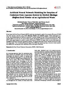
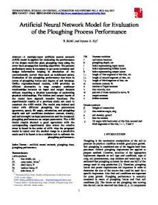
Time series plots of observed and predicted values of salinity at Murray Bridge with a lead time of 14-days obtained using the ANN with the 11 inputs selected using the modified PMI algorithm introduced in this paper are shown in Figures 1 and 2. It can be seen that the model performs extremely well for the training, testing and validation periods (Figure 1). Performance for the real-time forecasting simulation period was also very good, with the exception of the periods of uncharacteristic data identified by Bowden et al. (2002) (Figure 2).
Bowden, G.J., Maier, H.R. and Dandy, G.C. (2005), Input determination for neural network models in water resources applications. Part 2. Case study: forecasting salinity in a river, Journal of Hydrology, 301, 93- 107 Bowden, G.J., Maier, H.R. and Dandy, G.C. (2002), Optimal division of data fro neural network models in water resources applications, Water Resources Research, 38(2), 10.1029/2001 WR000266
The performance of the model developed in this study, as well as that of the models developed in previous studies, is shown in Table 4 in terms of root mean square error (RMSE). It should be noted that Bowden et al. (2005) used different techniques for data division, and hence direct comparison between the results for calibration and validation could not be conducted for the models with 13 and 21 inputs. It can be seen that the model with the 11 inputs identified using the modified PMI algorithm introduced in this study performs best overall, while also being the most parsimonious.
Chernick, M.R. (1999), Bootstrap Methods: A Practitioner’s Guide, Wiley, New York Davies, L. and Gather, U. (1993), The identification of multiple outliers, Journal of the American Statistical Association, 88 (423), 782 - 792 Fraser,
7.
Train 38 36
A.M. and Swinney, H.L. (1986), Independent coordinates for strange attractors for mutual information, Physical Review A, 33(2), 1134 – 1140
Pearson, R.K. (2001), Exploring process data, Journal of Process Control, 11, 179 – 194
Table 4. Performance of ANN models with different inputs ANN 51-30-1 13-32-1 21-33-1 11-20-1
REFERENCES
Phoon, K.K., Islam, M.N., Liaw, C.Y. and Liong, S.Y. (2002) Practical Inverse Approach for Forecasting Nonlinear Hydrological Time Series, Journal of Hydrological Engineering, 7(2), 116 – 128
RMSE (EC units) Test Valid Real-Time 52 59 86 95 113 35 50 87
Maier, H.R. and Dandy, G.C. (1996), The use of artificial neural network for the prediction of water quality parameters, Water Resources Research, 32(4), 1013 – 1022 Moon, Y.I., Rajagopalan, B. and Lall, U. (1995), Estimation of mutual information using kernel density estimators, Physical Review E, 52(3), 2318 – 2321
SUMMARY AND CONCLUSIONS
In this paper, a modified version of the PMI algorithm for input identification introduced by Sharma (2000) and modified by Bowden et al. (2005) is introduced. In the proposed algorithm, use of the 95th percentile confidence level as the stopping criterion for input selection, which is generally obtained by bootstrapping, is replaced with an outlier detection statistic, the Hampel distance. The proposed stopping criterion is considered to be more robust and computationally efficient than bootstrapping. This is confirmed by the results obtained from two non-linear test functions, as well as a real-life application. However, the utility of the proposed approach requires further testing.
Scott,
D.W. (1992), Multivariate Density Estimation: Theory, Practice and Visualisation, Wiley, New York
Sharma, A. (2000), Seasonal to interannual rainfall probabilistic forecasts for improved water supply management: Part 1- A strategy for system predictor identification, Journal of Hydrology, 239, 232 – 239 Silverman, B.W. (1986), Density Estimation for Statistics and Data Analysis, Chapman and Hall, New York
1811
Specht, D.F. (1991), A General Regression Neural Network, IEEE Transactions on
Neural Networks, 2(6), 568 - 576
1400
Observed Predicted
Salinity (EC units)
1200 1000 800 600 400 200
Training
Testing
Validation
0 Jan-87 Jul-87 Jan-88 Jul-88 Jan-89 Jul-89 Jan-90 Jul-90 Jan-91 Jul-91 Jan-92 Time (Days)
Figure 1. Observed and predicted values of salinity at Murray Bridge with 14 days lead time for calibration and validation data
1400 Observed Predicted
Salinity (EC units)
1200 1000 800 600 400 200
0 Aug-92 Feb-93 Aug-93 Feb-94 Aug-94 Feb-95 Aug-95 Feb-96 Aug-96 Feb-97 Aug-97 Feb-98 Time (Days)
Figure 2. Observed and predicted values of salinity at Murray Bridge with 14 days lead time for real-time simulation data
1812