Jun 14, 2005 - Similarity Evaluation on Tree-structured Data. Rui Yang. Panos Kalnis. Anthony K. H. Tung+. School of Computing. National University of ...
Similarity Evaluation on Tree-structured Data Rui Yang
Panos Kalnis Anthony K. H. Tung+ School of Computing National University of Singapore {yangrui,kalnis,atung}@comp.nus.edu.sg + Contact Author
ABSTRACT Tree-structured data are becoming ubiquitous nowadays and manipulating them based on similarity is essential for many applications. The generally accepted similarity measure for trees is the edit distance. Although similarity search has been extensively studied, searching for similar trees is still an open problem due to the high complexity of computing the tree edit distance. In this paper, we propose to transform tree-structured data into an approximate numerical multidimensional vector which encodes the original structure information. We prove that the L1 distance of the corresponding vectors, whose computational complexity is O(|T1 | + |T2 |), forms a lower bound for the edit distance between trees. Based on the theoretical analysis, we describe a novel algorithm which embeds the proposed distance into a filter-and-refine framework to process similarity search on tree-structured data. The experimental results show that our algorithm reduces dramatically the distance computation cost. Our method is especially suitable for accelerating similarity query processing on large trees in massive datasets.
1.
INTRODUCTION
The use of tree-structured data in modern database applications is attracting the attention of the research community. Typical examples of huge repositories of rooted, ordered and labeled tree-structured data include the secondary structure of RNA in biology or the XML data on the web. In this paper, we study the structure similarity measure and similarity search on large trees in huge datasets. These problems form the core operation for many database manipulations (e.g., approximate join, clustering, k-NN classification, data cleansing, data integration etc). Our findings are useful in numerous applications including XML data searching under the presence of spelling errors, efficient prediction of the functions of RNA molecules, version management for documents, etc. Trees provide an interesting compromise between graphs
Permission to make digital or hard copies of all or part of this work for personal or classroom use is granted without fee provided that copies are not made or distributed for profit or commercial advantage, and that copies bear this notice and the full citation on the first page. To copy otherwise, to republish, to post on servers or to redistribute to lists, requires prior specific permission and/or a fee. SIGMOD 2005 June 14-16, 2005, Baltimore, Maryland, USA. Copyright 2005 ACM 1-59593-060-4/05/06 $5.00.
and the linear representation of data. They allow the expression of hierarchical dependencies where the semantics are specified implicitly by the relationship between their components; thus, the structure of the tree plays an important role in differentiating the data. The most commonly used distance measure on tree-structured data is the tree edit distance [23]. However, computing the tree edit distance can be very expensive both in terms of CPU cost and disc I/Os, rendering it impractical for huge datasets. In this paper, we utilize a structure transformation to develop a novel distance function for rooted, ordered, labeled trees based on both the structure and the content. We prove that the proposed distance function is a lower bound of the tree edit distance. The idea is similar to using a set of q-grams to bound the edit distance of strings and thus filter out dissimilar strings [19]. Given a string S, a q-gram is a contiguous substring of S of length q. If S1 and S2 are within edit distance k, S1 and S2 must share at least max(|S1 |, |S2 |) − (k − 1)q − 1 common q-grams. Similarly we characterize a tree as a set of q-level binary branches, and we show that two trees T1 and T2 are within edit distance k precisely when they share [4 ∗ (q − 1) + 1] ∗ k q-level binary branches. Furthermore, just as string edit distance can be tightened if the positions of the q-grams in the string are also taken into account [17, 5], so too tree-edit distance can be tightened by using information detailing the positions of q-level binary branches in the trees. By employing our distance function as the lower bound of the edit distance in the filter-and-refine framework, we can evaluate similarity queries in two steps: In the filtering step, the lower bound is used to filter out most objects which are not possible to be in the result. The remaining objects are candidates which are validated by the original complex similarity measure during the refinement step. This strategy greatly reduces the number of expensive distance computations in the original space. Summarizing, the contributions of our paper are: • We propose a transformation which maps tree-structured data with the edit distance measure to numerical vectors with the standard L1 distance. The method maintains the structure information of the original data. The novel distance is proved to be the lower bound of the general tree-edit distance. • We describe a generalization of our mapping method which approximates the tree-edit distance at different resolutions. • By adapting q-grams methods to use the lower bound
property of the new distance, we propose novel methods to embed it into the filter-and-refine framework to facilitate the processing of similarity search. • We present a set of experiments which compare the performance of our algorithm with the histogram filtration methods proposed in Ref. [7]. The rest of the paper is organized as follows: In Section 2 we provide the background and an overview of the related work. Section 3 presents the definition of the transformed vector space and the new distance based on it, together with the formal proof of the lower bound theorem. In Section 4 we discuss how to embed our distance function as the lower bound of edit distance into the framework for similarity search, while in Section 5 we present a thorough experimental study of our algorithms. Finally, Section 6 concludes our paper.
2.
PRELIMINARIES AND RELATED WORK
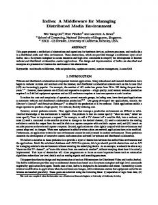
In this paper, we focus on the huge dataset D of rooted, ordered, labeled trees. Here, a tree is defined as a data structure T = (N, E, Root(T )). N is a finite set of nodes. E is a binary relation on N where each pair (u, v) ∈ E represents the parent-child relationship between two nodes u, v ∈ N . Node u is the parent of node v and v is one of the child nodes of u. There exists only one root note, denoted as Root(T ) ∈ N , which has no parent. Every other node of the tree has exactly one parent and it can be reached through a path of edges from the root. The nodes which have a common parent u (i.e., all the children of u) are siblings. |T | is the number of nodes in tree T , or the size of T . A rooted ordered tree is a tree in which the order of the siblings from left to right is significant. A rooted, ordered, labeled tree is an ordered tree structure T = (N, E, Root(T ), label), where label : N → Σ is a total function and Σ is the finite alphabet of vertex labels. In our paper, we focus on rooted ordered labeled trees. Fig. 1 is an example of two trees T1 and T2 .
2.1 Structural Similarity Measure The measure of similarity between two trees T1 and T2 has been well studied in combinatorial pattern matching. Most studies use edit distance to measure the dissimilarity between trees (notice that similarity computation is the dual problem of distance computation). Usually there are three kinds of basic edit operations on tree nodes [23]: (i) Relabeling means changing the label of nodes; (ii) Deleting a node n means assigning the children of n to be the children of the parent of n and removing n; (iii) Inserting node n under n� means assigning a consecutive subsequence of the children of n� as the children of n, and appending n under n� . As mentioned in Ref. [23], a mapping between two trees can specify the edit operations applied to each node in the two trees graphically. The mapping must be one-to-one and it must preserve the sibling order and ancestor order at the same time. If node u ∈ T1 is mapped to node v ∈ T2 and label(u) �= label(v), u is relabeled to v. If u ∈ T1 has no correspondence in the mapping, u is deleted. If v ∈ T2 has no correspondence in the mapping, v is inserted. For example, the mapping, represented by the dashed line in Fig. 1 shows a way to transform T1 to T2 . For the general case, functions γ(e) are defined to evaluate each edit operation e. The cost of a sequence of edit
� operations e1 , e2 , · · · , ek is ki=1 γ(ei ). The edit distance between T1 and T2 , denoted as EDist(T1 , T2 ), is defined as the minimum cost of edit operation sequences that can transform T1 to T2 . If the cost for each operation equals 1, the edit distance, referred to as unit cost tree edit distance, is the minimum number of operations required to transform one tree into the other. The unit cost edit distance is a distance metric and is adopted in this paper for its simplicity. However, our algorithm can be easily extended to the general edit distance measure if there is a lower bound on the cost for each edit operation. The main differences between various tree edit distance algorithms lie in the set of allowed edit operations. Earlier work allows insertion and deletion of single nodes at the leaves only and relabeling of nodes anywhere in the tree [14]. The definitions in Ref. [23, 16, 18, 22] allow insertion and deletion of single nodes anywhere in a tree. In Ref. [22] a new distance metric based on a restriction of the mappings between two trees is proposed. The intuition is that two separate sub-trees of T1 should be mapped to two separate subtrees in T2 . In Ref. [18], on the other hand, insertion is allowed only before deletion. Dynamic programming algorithms are frequently used to solve the edit distance problem. To the best of our knowledge, the most commonly cited algorithm to compute general edit distance between rooted ordered labeled trees appears in Ref. [23]. The algorithm runs in O(|T1 ||T2 |) space and O(|T1 ||T2 | min(depth(T1 ), leaves(T1 )) min(depth(T2 ), lea ves(T2 ))) time, where depth(Ti ), leaves(Ti ), i = 1, 2 are the depth and the number of leaf nodes of tree Ti respectively. In the worst case, the time complexity of the algorithm is O(|T1 |2 |T2 |2 ). Obviously, the tree-edit distance computation is both CPU and I/O expensive and is not scalable for similarity search on large trees in huge datasets.
2.2 Related Work on Tree Similarity Although similarity search on numerical multidimensional data has been extensively studied [6, 12, 2, 20, 13], similarity search on tree-structured data has only recently attracted the attention of the research community [7]. As mentioned above, similarity evaluation of tree structured data in massive datasets based on the tree-edit distance is expensive both in terms of CPU and I/O cost; therefore, most of the previous work utilizes the filter-and-refine approach. To guarantee the filtration efficiency, the lower bound function should be a relatively precise approximation of the tree-edit distance. At the same time, it should be computationally much less expensive than the real distance. The authors of Ref. [15] proposed a pivot based approximate similarity join algorithm on XML documents. In their method, XML documents are transformed into their corresponding preorder and postorder traversal sequences. Then the maximum of the string edit distance of the two sequences is used as the lower bound of the tree-edit distance. They also proposed additional heuristics to reduce the amount of edit-distance computations between pairs of trees. However, the complexity of computing the proposed lower bounds is still O(|T1 ||T2 |) (i.e., the complexity of sequence edit distance computation), and it is not scalable to our problem. In order to correlate XML data streams, Garofalakis et.al. [4] proposed embedding the tree-edit distance metrics (allowing a move operation in addition to the basic operations) into a numeric vector space with L1 distance norm. In their method, XML
trees are hierarchically parsed into valid subtrees in different phases. Then the multi-set of valid subtrees is obtained by parsing the tree. The vector representation is defined as the characteristic vector of the multi-set. The L1 distance of the vectors guarantees an upper bound of distance distortion between two trees. However, the method fails to give a constant lower bound on the tree-edit distance to facilitate the retrieval of exact answers to the similarity queries based on similarity measure. In their recent work, Kailing et.al. [7] presented a set of filters grounded on structure and content-based information in trees. They proposed using the vectors of the height histogram, the degree histogram and the label histogram to represent the structure as well as content information of trees. The lower bound of the unordered-tree edit distance can be derived from the L1 distance among the vectors. They also suggested a way to combine filtration to facilitate similarity query processing. However, their filters are for unordered trees and cannot explore the structure information implicitly depicted by the order of siblings. Moreover, their lower bounds are obtained by considering structure and content information separately. In our approach, we suggest combining the two sources of information to provide accurate lower bounds for the tree-edit distance. In Section 5 we compare the performance of our algorithm against the histogram filtration methods.
2.3 Binary Tree Representation of Forests (or Trees) Our proposed mapping of tree structures into a numeric vector space is based on the binary tree representation of rooted ordered labeled trees. For completeness, we briefly describe the binary tree representation of forests (or trees). We cite the formal definition of the binary tree from Ref. [9]: Definition 1 (Binary Tree) A binary tree consists of a finite set of nodes. It is: 1. an empty set. Or 2. a structure constructed by a root node, the left subtree and the right subtree of the root. Both subtrees are binary trees, too. In a binary tree, the edges between parents and the left child nodes are different from those between parents and the right child nodes. We use TB = (N, El , Er , Root(T )) to represent a binary tree. ∀u, v1 , v2 ∈ N , if v1 (v2 resp.) is the left (right resp.) child of u, then �u, v1 �l ∈ El (�u, v2 �r ∈ Er resp.). A full binary tree is a binary tree in which each node has exactly zero or two children. There is a natural correspondence between forests and binary trees. The standard algorithm to transform a forest (or a tree) to its corresponding binary tree is through the left-child, right-sibling representation of the forest (tree): (i) Link all the siblings in the tree with edges. (ii) Delete all the edges between each node and its children in the tree except those edges which connect it with its first child. Note that the transformation does not change the labels of vertices in the tree. We can transform1 T1 and T2 of Fig. 1 into B(T1 ) 1 The appended nodes labeled ε and the numbering of the nodes are explained in sections 3.2 and 4.2, respectively.
and B(T2 ) shown in Fig. 2, respectively. The binary tree representation is denoted as B(T ) = (N, El , Er , Root(T ), label) in our paper. a
b
c
a
c
d
d
c
d
e
d
b c
e
b
b
e T1
T2
Figure 1: Tree Examples a(1,8)
a(1,9)
b(2,3)
b(2,5)
ε b(5,6)
c(3,1) ε
ε
e(8,7)
c(6,4)
d(4,2) ε
ε
ε
d(7,5) ε
ε
B(T1)
ε
c(3,1) ε ε
c(7,6)
d(4,2) ε
ε
d(8,7) ε
b(5,4)
e(6,3) ε
ε
e(9,8) ε
ε
ε B(T2)
Figure 2: Normalized Binary Tree Representation
3. TREE STRUCTURE TRANSFORMATION The key element of our algorithm is to transform rooted, ordered, labeled trees to a numeric multi-dimensional vector space equipped with the norm L1 distance. The mapping of a tree T to its numeric vector ensures that the features of the vector representation retain the structural information of the original tree. Furthermore, the tree-edit distance can be lower bounded by the L1 distance of the corresponding vectors. The lower bound distance evaluation is computationally much less expensive than that of EDist(T, T � ). In this section, we present the transformation methods and the proof of the lower bound theorem.
3.1 Observation We observe that edit operations change at most a fixed number of sibling relationships. This is because each node in a tree can have a varying number of child nodes but at most two immediate siblings. This is illustrated in the example of Fig. 1. The deletion of node b in T1 incurs five changes in parent-child relationships: It destroys the (a, b), (b, c), (b, d) edges, while generating the (a, c), (a, d) edges. At the same time, this edit operation only incurs four changes in sibling relationships: The one between b and b, and the one between b and e are destroyed. The sibling relationship between b and c, and the one between d and e are generated by the deletion operation. As mentioned in 2.3, a binary tree corresponding to a forest retains all the structure information of the forest. Particularly, in the binary tree representation, the original parentchild relationships between nodes, except the ones between each inner nodes and its first child, are removed. The removed parent-child relationships are replaced by the link
edges between the original siblings. This property makes the transformed binary tree representation appropriate for highlighting the effect of the edit-based operations on original trees.
3.2 Vector Representation of Trees To encode the structural information we normalize the transformed binary tree representation B(T ) of T . In B(T ), for any node u, if u has no right (or left) child, we append a � node (i.e., nodes labeled as � do not exist in T ) as u’s right (or left) child. Thus we make T a full binary tree in which all the original nodes have two children and all the leaves are labeled as � (as in Fig. 2). The normalized binary tree representation is defined as B(T ) = � (N {�}, El , Er , Root(B(T )), label), where � denotes the appended nodes as well as their labels. To simplify the notation, in this paper u ∈ N represents the node as well as its label where no confusion arises. In order to quantify change detection in a binary tree, we define the binary branch on normalized binary trees: Definition 2 (Binary Branch) Binary branch (or branch for short) is the branch structure of one level in the binary tree. For a tree T , ∀u ∈ N there is a binary branch BiB(u) in B(T ) such that BiB(u) = (Nu , Eul , E �ur , Root(Tu )), where Nu = {u, u1 , u2 } (u ∈ N ; ui ∈ N {�}, i = 1, 2), Eul = {�u, u1 �l }, Eur = {�u, u2 �r } and Root(Tu ) = u in the normalized B(T ). According to the properties of normalized binary trees, we have Lemma 3.1: Lemma 3.1 For each node u ∈ N of a tree T , u may appear in at most two binary branches in the binary tree representation B(T ). PROOF: 1. u can occur as root in at most one binary branch. This is obvious. 2. u can occur as the left (or right) child in at most one binary branch. u can not occur as the left child in one branch and as the right child in another branch at the same time; otherwise, u must have two parents in B(T ). That is contrary to the properties mentioned in section 2. Assume that the universe of binary branches BiB() of all trees in the dataset composes alphabet Γ and the symbols in the alphabet are sorted lexicographically on the string uu1 u2 . A representative vector of dimension |Γ| can be built for each tree-structured data record, with each dimension recording the number of occurrences of a corresponding branch in the data. The formal definition of the binary branch vector is given in Definition 3. Definition 3 (Binary Branch Vector) The binary branch vector BRV (T ) of a tree T is a vector (b1 , b2 , · · · b|Γ| ), with each element bi representing the number of occurrences of the ith binary branch in the tree. |Γ| is the size of the binary branch space of the dataset. We can first build an inverted file for all binary branches, as shown in Fig. 3(a). An inverted file has two main parts:
a vocabulary which stores all distinct values being indexed, and an inverted list for each distinct value which stores the identifiers of the records containing the value. The vocabulary here consists of all existing binary branches in the datasets. The inverted list of each component records the number of occurrences of it in the corresponding trees. The resulting vectors of our transformation for the trees in Fig. 1 and the normalized binary trees in Fig. 2 are shown in Fig. 3(b). a . b . b . b . b . c . d . d . d . e . b .. b .. c .. c .. e .. ε .. ε .. ε .. ε .. ε .. ε c d b e ε ε c e ε T1 2
T1 1
T1 1
T1 1 T2 1
T2 1
T2 2
T2 1
T1 1
T1 2 T2 1
T2 1
T2 2
(a) Inverted File BRV(T1)
1
...
1
...
0
...
1
...
0
...
2
...
0
...
0
...
2
...
1
...
BRV(T2)
1
...
0
...
1
...
0
...
1
...
2
...
1
...
1
...
0
...
2
...
(b) Binary Branch Vectors
Figure 3: Binary Branch Vector Representation Based on the vector representation, we define a new distance of the tree structure as the L1 distance between the vector images of two trees: Definition 4 (Binary Branch Distance) Let BRV (T1 ) = (b1 , b2 , · · · , b|Γ| ), BRV (T2 ) = (b�1 , b�2 , · · · b�|Γ| ) be the binary branch vectors of trees T1 and T2 respectively. The binary |Γ| branch distance of T1 and T2 is BDist(T1 , T2 ) = Σi=1 |bi −b�i | The binary branch distance has the properties listed below: For all T1 , T2 and T3 in the dataset, 1. BDist(T1 , T2 ) ≥ 0, and BDist(T1 , T1 ) = 0 2. BDist(T1 , T2 ) = BDist(T2 , T1 ) 3. BDist(T1 , T3 ) ≤ BDist(T1 , T2 ) + BDist(T2 , T3 ) PROOF The first two properties are obvious. For the third property, let BRV (Ti ) = (bi1 , bi2 , · · · , bi|Γ| ) for i = 1, 2, 3. BDist(T1 , T2 ) + BDist(T2 , T3 ) |Γ| |Γ| = Σj=1 |b1j − b2j | + Σj=1 |b2j − b3j | |Γ| ≥ Σj=1 |b1j − b3j | = BDist(T1 , T3 )
The third property means that the binary branch distance satisfies the triangular inequality. However, BDist(T1 , T2 ) = 0 cannot imply that T1 is identical to T2 . This is illustrated in Fig. 4, where both trees have the same binary branch vector. So the binary branch distance is not a metric on tree-structured data.
A
A
B
c
B
C
C
...
w1
D
...
C
D
v’
v’
w2
...
w2
...
wl w l+1
Figure 4: Trees with 0 Binary Branch Distance
...
...
w l+m
2. Assume that ej inserts a node v to transform Tj−1 to Tj . Obviously, when v has a parent, a left sibling, a right sibling and child nodes, this operation leads to the maximum number of changes on the structure information. Fig. 5 and Fig. 6 demonstrate the insertion operation and the changes it causes on the binary tree representation. Let v be inserted under node v � and child nodes wl+1 , · · · wl+m of v � in Tj−1 become the child nodes of v in Tj .
... ...
v’
...
...
wl
w l+m ...
w l+m+1
...
w1
w2
...
...
v
wl
w l+m+1
...
... ...
w l+1
w l+m+1 ... ...
w l+m
1. Assume that ei is a relabeling operation on some node v of the tree. According to Lemma 3.1, v occurs in at most two binary branches in B(Ti−1 ). In these two branches, label(v) is changed to the new one in the target tree B(Ti ). Assume that the count of the two binary branches in BRV (Ti−1 ) is in dimension l1 and l2 , while the two new binary branches are in dimension l3 and l4 . Then BRV (Ti−1 )[lm ] − BRV (Ti )[lm ] = 1, for m = 1, 2. BRV (Ti−1 )[lm� ] − BRV (Ti )[lm� ] = −1, for m� = 3, 4. So, BDist(Ti−1 , Ti ) ≤ 4.
w2
v ...
w l+2 ...
Theorem 3.2 Let T and T � be two trees. If the tree-edit distance between T and T � is EDist(T, T � ), then the binary branch distance between them satisfies the following: BDist(T, T � ) ≤ 5 × EDist(T, T � ) PROOF: The theorem follows if we show that at most 5 × k binary branch distance is incurred by k edit operations. Assume that edit operations e1 , e2 , · · · , ek transform T to T � . Accordingly, there is a sequence of trees T = T0 → T1 → · · · → Tk = T � , where Ti−1 → Ti via ei for 1 ≤ i ≤ k. Let there be k1 relabeling operations, k2 insertions and k3 deletions. k1 + k2 + k3 = k. It is sufficient to prove the theorem for one step of the transformation.
w1
wl w l+1
In this section, we prove our main theorem.
v’
... ...
w l+m+1
3.3 Lower Bound of Edit Distance
...
w1
w l+m
Figure 5: Insertion of Node v Under Node v � We show that at most five changes occur on the edges of B(Tj−1 ): Two edges �v, wl+1 �l and �v, wl+m+1 �r representing the structure information rooted on v are added into the binary tree. These edges comprise the binary branch BiB(v). So, assuming that it corresponds to dimension l in BRV (Tj ), then BRV (Tj )[l]− BRV (Tj−1 )[l] = 1. In addition, the sibling relationship between wl and wl+1 , and between wl+m and wl+m+1
...
Figure 6: Changes of Binary Tree Incurred by Insertion in Tj−1 (represented by �wl , wl+1 �r and �wl+m , wl+m+1 �r respectively in B(Tj−1 )) are destroyed. This leads to the destruction of one of each binary branch BiBTj−1 (wl ) and BiBTj−1 (wl+m ). Thus, the values for the two corresponding dimensions in BRV (Tj ) are less than those in BRV (Tj−1 ) by 1. Finally, �wl , wl+1 �r is replaced by �wl , v�r in B(Tj ) for v is the right sibling of wl after being inserted in Tj . �wl+m , wl+m+1 �r is replaced by �wl+m , ��r for wl+m is the right most child of v in Tj after insertion. Then the values of the corresponding two dimensions in BRV (Tj ) are larger than those in BRV (Tj−1 ) by 1 each. To sum up, BDist(Tj−1 , Tj ) is at most 5. 3. Deletion is complementary to insertion. Therefore the number of affected binary branches must be bounded by the same amount as for insertion. According to the triangular inequality property of binary branch distance, we have BDist(T, T � ) ≤ BDist(T0 , T1 ) + BDist(T1 , T2 ) + · · · +BDist(Tk−1 , Tk ) ≤ 4 × k1 + 5 × k2 + 5 × k3 ≤ 5 × k ≤ 5 × EDist(T, T � ).
3.4 Extended Study Our generalized analysis is similar to the q-gram method [19] for solving the k-difference problem of strings. The number of occurrences of each q-gram (i.e., all strings of length q over the alphabet) in any two strings are counted. If two strings are similar, they have many q-grams in common. Formally, if the edit-distance of strings S1 and S2 is k, then they have at least max(|S1 |, |S2 |) − (k − 1)q − 1 q-grams in common. When applied to similarity search problems in which the full strings are involved, the q-gram method usually trades off the false positive for the false negative rate by adjusting the length of the q-gram searched [8]. Binary branches can be viewed as playing the role of q-gram structures for tree data. The vector images of trees can be extended to record multiple level binary branch profiles. We first give the formal definition of the q-level binary branch: Definition 5 The q-level binary branch BiB Q(n0 , n1 , · · · , n2q −2 ) is the perfect binary tree of height q − 1, where n0 , n1 , · · · , n2q −2 is the sequence obtained by preorder traversing the perfect binary tree (with all leaf nodes at the same depth and all internal nodes having degree 2).
The binary branch defined in the previous section is indeed the two-level binary branch. Similar to the computation of q-grams for strings, our sliding window is a perfect binary tree with height q − 1. The sliding window shifts one level each time along the path from the root to the leaves. For each node u in the tree, there is a q-level binary branch rooted at u in the binary tree representation. If the subtree of height q − 1 rooted at u is not a perfect binary tree in the transformed representation, we can append �-nodes to complete it. The multiple level binary branch is used to maintain structures of fixed size and fixed shape in the original data. Obviously, it encodes more information than the two-level binary branch. We can extend the binary branch vector to the characteristic vector BRV Q(T ), which includes all the elements in the q-level binary branch space. The q-level binary branch distance BDist Q(T, T � ) is defined as the L1 vector distance between the images of the trees T and T � under the q-level mapping. Theorem 3.3 Let T and T � be two trees. If the tree-edit distance between T and T � is EDist(T, T � ) = k, then the qlevel binary branch distance between them BDist Q(T, T � ) ≤ [4 × (q − 1) + 1] × k The proof methods here are similar to those of Theorem 3.2. Note that each node in T appears in at most q q-level binary branches in B(T ). We do not include the details of the proof due to space constraints. The binary branch distance BDist Q(T1 , T2 ) increases as the level of the binary branch q increases. This is due to the fact that the higher the level is, the more information of the tree structure is encoded in the binary branches. At one extreme, q is equal to the height of the normalized transformed binary tree; then all the structural information of the original tree is encoded. However, in such a situation, the filter algorithm is of no use. At the other extreme q is equal to 1; in this case, the filter efficiency is too low. We do not discuss this option as it records no structure information of the original tree at all. According to Theorem 3.3, BDist Q(T, T � )/[4(q − 1) + 1] can be used as a series of approximations for the tree-edit distance with different resolutions. So the level q of the binary branch can be adjusted to improve filter efficiency when solving the similarity search problem.
4.
ENHANCEMENT OF SIMILARITY SEARCH
Previously, we mapped the tree structures and the tree edit distance metric to a numeric vector space and the L1 norm distance. Although, according to its properties, the binary branch distance is not a metric, it approximates and lower bounds the tree-edit distance metric. Just as q-gram methods can be used to speed up similarity search for strings, the distance-embedded lower bounds can be integrated into the filter-and-refine framework to speed up similarity search by reducing the number of expensive similarity distance computations. In this section, we present our filter-and-refine algorithm for processing similarity search on the tree-structured data by exploiting the lower bounds.
4.1 Basic Algorithm Similarity search on various data usually refers to range queries and k nearest neighbor queries. Range queries find
all objects in the database which are within a given distance τ from a given object; k nearest neighbor (k-NN) queries find the k most similar objects in the database which are closest in distance to a given object. Other types of search can be composed by these two similarity queries. When searching tree-structured data, similarity is measured by tree-edit distance. As mentioned above, the similarity evaluation of large trees in massive datasets based on tree-edit distance is a computationally expensive operation. Traditionally, the filterand-refine architecture is utilized to reduce real distance computation by employing the lower bounds of the real distance [13]: In the first step (i.e., filtration), objects that cannot qualify are filtered out. In the second step (i.e., refinement), verification of the original complex similarity measure is necessary only for the candidates filtered through. The objects satisfying the query predicate are reported as results. The completeness of the results is guaranteed by the lower bound property: If the lower bound distance is greater than the query range, it is safe to filter out the data since its real edit distance cannot be less than that range. Our method is to embed an easy-to-compute distance function that is the lower bound of the actual tree edit distance into the filter-and-refine framework. The optimistic bound used by the similarity search is based on the binary branch vector distance of the trees. In addition to the number of occurrences of individual binary branch, the positional information of the binary branch is also important in exploring the structure information of the trees. We will focus on the two-level binary branch. However, our approach can be easily generalized to q-level binary branches.
4.2 Optimistic Distance for Similarity Queries The efficiency of the filter-and-refine architecture is based on the hypothesis that the lower bound function is much quicker to evaluate than real distance. As shown in Section 3.3, binary branch distance lower bounds edit distance effectively: The lower bound function can be computed in O(|T | + |T � |) time, which is much more succinct than edit distance computation. Like using the q-gram methods to solve the approximate string matching problem, not only the occurrences of the q-grams, but also their positions can be exploited to measure the similarity of the pattern and certain subsequence of the strings [17, 5]. The idea is that: given two strings with distance less than l, two identical qgrams in the two strings respectively cannot be matched if their positions differ by more than l. Binary branch filtration also exhibits this property. First, we give the following proposition: Proposition 4.1 Given T1 and T2 with edit distance less than l, we number each node u by its position in the preorder traverse of its tree. In the mapping corresponding to the edit distance, the node u ∈ T1 cannot be mapped to v ∈ T2 if the difference of the numbers of u and v is larger than l. PROOF(sketch): In the preorder traversal numbering, the numbers which are smaller than that of u are assigned to ancestors of u or the nodes that are to the left of u, while the ones that are larger than that of u are assigned to descendants or the nodes to the right of u. Since the edit operation mapping preserves sibling order and ancestor order, if the two nodes are matched, and their number difference is larger than l, then there must be more than l deletions
or insertions. This is contrary to the premise that the edit distance is less than l. The property is also applicable to postorder numbering of the nodes. For each binary branch BiB(u, u1 , u2 ), we define the positional structure (BiB(u, u1 , u2 ), pre(u), post(u)), where pre(u) and post(u) denote the position of u in the preorder and the postorder traversal sequence of T respectively (resp. the preorder traverse and inorder traverse of B(T )). Based on the positional binary branch, we define the mapping M (T1 , T2 , pr) between the positional binary branches of T1 and T2 with positional range pr, which is any set of pairs of positional binary branches ((BiB(u, u1 , u2 ), pre(u), post(u)), (BiB(v, v1 , v2 ), pre(v), post(v))) satisfying: 1. the mapping is one-to-one; 2. BiB(u, u1 , u2 ) = BiB(v, v1 , v2 ); 3. |pre(u) − pre(v)| ≤ pr and |post(u) − post(v)| ≤ pr. For the example in Fig. 2, the numbering beside each node is the position specification of the corresponding binary branch. Assume the positional range pr = 1. It is obvious that (BiB(c, �, d), 3, 1) in T1 can only be mapped to (BiB(c, �, d), 3, 1) in T2 ; While (BiB(c, �, d), 6, 4) and (BiB(c, �, d), 7, 6) cannot be mapped to each other. (BiB(e, �, �), 8, 7) in T1 can be mapped to (BiB(e, �, �), 9, 8) in T2 , but cannot be mapped to (BiB(e, �, �), 6, 3). For two trees T1 and T2 , we denote the maximum-sized mapping as Mmax (T1 , T2 , pr). The subset of it which is related to a given binary branch BiB ∈ Γ is denoted as � � (T1 , T2 , BiB, pr). Obviously, Mmax (T1 , T2 , BiB, pr) is Mmax the maximum-sized mapping on the binary branch BiB. Given the preorder and postorder position sequences of BiB � (T1 , T2 , BiB, pr)| in T1 and T2 in ascending order, |Mmax � (size of Mmax (T1 , T2 , BiB, pr)) can be computed in linear time. We define a new distance between two trees based on � |Mmax (T1 , T2 , BiB, pr)|: Definition 6 (Positional Binary Branch Distance) Given two trees T1 and T2 , their binary branch vectors BRV (Ti ) = (bi1 , bi2 , · · · , bi|Γ| ) (i = 1, 2) and the positional range specification pr, the positional binary branch distance with range �|Γ| � pr is P osBDist(T1 , T2 , pr) = j=1 (b1j +b2j −2|Mmax (T1 , T2 , j, pr)|) Proposition 4.2 If P osBDist(T1 , T2 , l) > 5×l, then EDist (T1 , T2 ) > l. PROOF(sketch): We prove the contrapositive proposition: If the edit distance is less than l, then P osBDist(T1 , T2 , l) ≤ 5 × l. According to the definition of positional binary branch, P osBDist(T1 , T2 , l) differs from BDist in that, in T1 and T2 , it does not match the same binary branches whose position differences are larger than l. For any positional binary branch (BiB(u, u1 , u2 ), pre(u), post(u)), if there is no element in Mmax (T1 , T2 , l) that corresponds to it, the node u should be changed by some edit operation. According to Definition 6, the positional binary branch distance is the sum of the differences on the binary branch incurred by the edit operations to change T1 to T2 . And according to Theorem 3.2, one edit operation changes at most 5 binary branches. Thus P osBDist(T1 , T2 , l) ≤ 5 × l.
Obviously the positional binary branch distance is related to the positional range specification. Theoretically, the positional range for two trees T1 and T2 can increase from prmin = 0 to prmax = |T1 | + |T2 | and the positional binary branch distance decrease correspondingly. Given pr = prmin , the corresponding positional binary branch distance computed has the maximum possible value: P osBDist(T1 , T2 , prmin ) = P osBDistmax , computed by matching only the identical binary branches which have the same positions. Apparently, P osBDistmax /5 > prmin . Given pr = prmax , the corresponding positional binary branch computed has the minimum possible value P osBDist(T1 , T2 , prmax ) = P osBDistmin = BDist (T1 , T2 ). It is obvious that P osBDistmin /5 ≤ EDist(T1 , T2 ) ≤ prmax
Then, there must be a given positional range pri s.t. prmin ≤ pri ≤ prmax which is the maximum positional range that satisfies P osBDist(T1 , T2 , pri )/5 > pri . According to the analysis of Proposition 4.2, EDist(T1 , T2 ) ≥ (pr +1), where pr = prmin , · · · , pri . Thus, (pri + 1) is a lower bound of edit distance. Note that BDist(, ) is the minimum value for P osBDist and that for pri + 1, P osBDist(T1 , T2 , pri + 1)/5 ≤ (pri + 1), so we have: BDist(T1 , T2 )/5 ≤ P osBDist(T1 , T2 , pri + 1)/5 ≤ (pri + 1)
Thus, pri + 1 is a closer lower bound of edit distance between T1 and T2 than BDist(T1 , T2 )/5. A better optimistic bound, propt , of the edit distance can be obtained by searching the minimum value of the positional range pri (prmin ≤ pri ≤ prmax ) satisfying P ostBDist(T1 , T2 , pri )/5 ≤ pri . In practice, we can reduce the search range further. Since EDist(T1 , T2 ) ≥ ||T1 | − |T2 ||, prmin = ||T1 | − |T2 ||. At the same time, it is meaningless to set the prmax to be larger than max(|T1 |, |T2 |);
4.3 Similarity Search Algorithm In this section, we present the algorithm for constructing vectors and a novel filter-and-refine algorithm for similarity search utilizing the positional binary branch distance. The steps of vector construction and k-NN search are listed in Algorithm 1 and Algorithm 2 respectively. In the vector construction algorithm, we utilize an extended inverted file IF I to build the vector representation. The inverted list of each binary branch records the data record T id, the number of occurrences of this branch and the respective positions at which it appears in the corresponding data. Firstly, each tree-structured data is recursively traversed and the IF I is constructed by calling the function T raverse( ) to obtain the binary branch information in Fig. 2. In the function, the binary branch BiBR of the current node is built by calling the getF irstChild() and getN extSibling() functions of the parser. Then, in function insertP reOrder( ), the corresponding entry of BiBR in IF I is found by some hashing function. Then the component for data T (identified by T id) at the end of inverted list is updated: The number of occurrences is increased by 1. The preorder position of the branch is recorded. In function insertP ostOrder( ), the postorder position is recorded. After the construction of IF I, we build the sparse vector representation of each data by scanning IF I: For each branch that occurs in the data, we record the id of the branch and the number of its occurrences in the vector. In addition, two arrays recording the branch positions (for preorder and
Algorithm 1 vector construction
Algorithm 2 k-NN on tree-Structured data
Input: The data set D Output: The vector representations of the data BRV , The preorder positions preOrderP os, The postorder positions postOrderP os, 1: initialize the inverted file index IF I to be empty; 2: for each record T ∈ D do 3: P reP osition = 0; 4: P ostP osition = 0 ; 5: T raverse(Root(T ), P reP osition, P ostP osition, IF I); 6: l = 0; 7: for each entry i in IF I do 8: for each entry j in the inverted list of i do 9: k = IF I[i][j].T id; 10: BRV [k][l].Bib ← i; 11: BRV [k][l + +].Count ← IF I[i][j].occurrence; 12: Build positional sequence preOrderP os[k]; 13: Build positional sequence postOrderP os[k];
Input: The data set D, The vector representation of data BRV , The preorder positions preOrderP os, The postorder positions postOrderP os, The query Tq ; Output: The result set of k nearest neighbors of Tq 1: construct vector and position arrays vecTq , preOrderP osTq and postOrderP osTq for Tq ; 2: for each vector i in BRV do 3: LowerBound[i] = SearchLBound(vecTq , BRV [i], preOrderP os[i], postOrderP os[i], preOrderP osTq , postOrderP osTq ); 4: sort the LowerBound and D into LowerBound� and D� in ascending order of the lower bound distances; 5: initialize the max heap KN N , s.t. capacity(KNN)=k; 6: for i From 0 To |D| do 7: if (KN N.size = k)AND(LowerBound� [i] >KN N [0].key) then 8: BREAK; 9: Retrieve the corresponding data Ti ; 10: editDist = EDIST (Ti , Tq ); 11: if KN N.size is less than k then 12: insert Ti with the key editDist in KN N ; 13: else 14: pop up KN N [0]; 15: insert and push down Ti with the key editDist in KN N ; 16: return KN N ;
Function: T raverse(R, & P reorder, & P ostorder, IF I) 1: construct binary branch BiBR of R by calling getF irstChild(R) and getN extSibling(R); {two level binary branch} 2: P reorder++; 3: insertP reOrder(T id, BiBR , IF I, P reorder); 4: for each child node ri of R do 5: T raverse(ri , P reorder, P ostorder, IF I); 6: P ostorder++; 7: insertP ostOrder(T id, BiBR , IF I, P ostorder);
postorder respectively) are constructed from IF I. Both are sorted according to the branches and in ascending order. The procedure for k-NN search is shown in Algorithm 2. First, the query Tq is preprocessed to construct the vector representation and position sequences. In line 3, the optimistic bound of the distance between the query and each data object is computed by calling function SearchLBound; In the function, the optimistic bound is searched for in the range [dif f (size(vecTq ), size(BRV [i])), max(size(vecTq ), size(BRV [i]))]. Since the search range is ordered, we use the binary search algorithm. In line 3 and line 8 of function SearchLBound( ), the distance P osBDist() are com� ()|. After the optimistic bounds of puted based on |Mmax all the vectors are obtained, at line 4 of the main function, the LowerBound array and the data tree id are sorted in ascending order of the optimistic bounds to ensure that vectors of high possibility in being the results are processed before others. Second, the pruning procedure of traditional filterand-refine similarity search steps are adopted [13, 1, 10, 11] to reduce real distance computation. Finally, refinements are done by verifying the candidates. Range query processing is similar to k-NN query processing; The difference is that there is a specified range τ for the query. According to Proposition 4.2, max(P osBDist(T, Tq , τ ) /5, propt ) should be considered as the optimistic bound in the filtering step.
4.4 Complexity Analysis In this part, we analyze the time and space complexities of our vector construction method and optimistic bound computation method. In order to calculate running time complexity, we consider each step of the algorithm. Assume that the size of the dataset, i.e., the total number of tree
Function:SearchLBound(vecTq , BRVi , preOrderP osi, postOrderP osi, preOrderP osTq , postOrderP osTq )
1: prmin = dif f (size(vecTq ), size(BRVi )); 2: prmax = max(size(vecTq ), size(BRVi )); 3: P osBDistmax = P osDif f (vecTq , BRVi , preOrderP osi, postOrderP osi, preOrderP osTq , postOrderP osTq , prmin );
4: if P osBDistmax /5 ≤ prmin then 5: Return prmin ; 6: while prmin ≤ prmax do 7: prhalf = (prmin + prmax )/2; 8: P osBDist = P osDif f (vecTq , BRVi , preOrderP osi, postOrderP osi , preOrderP osTq , postOrderP osTq , prhalf );
9: if P osBDist/5 ≤ prhalf then 10: prmax = prhalf − 1; 11: else 12: prmin = prhalf + 1; 13: Return prhalf + 1;
data objects, is |D|. For record Ti , there are |Ti | nodes in it. The vocabulary of inverted file IF I is implemented by one hashing function. According to Algorithm 1, function T raverse() is called recursively to traverse each node and insert the binary branch information of the current node into IF I. Each time the new entries are appended at the end of the inverted list. So each update of IF I is of constant time complexity. Thus, the IF I construction is of linear complexity. As we store in IF I only the existing vocabulary of the dataset, the worst case is that all the nodes in the datasets have got different binary branches. Thus, the size of the � vocabulary is at most |D| i=1 |Ti |. In addition, each node in each tree has one corresponding entry in the inverted list. � In total, the space complexity of IF I is also O( |D| i=1 |Ti |). To build the vector representation, the whole IF I has to be scanned once. So the time and space complexities of the � whole vector construction algorithm are both O( |D| i=1 |Ti |). Next, we analyze the optimistic bound computation com-
plexity in our query processing method. Given one query Tq , we need to compare its vector and its positional sequence with those of each data Ti . As mentioned in section 4.3, we use the binary search algorithm to obtain the optimistic bound between ||Ti |−|Tq || and max(|Ti |, |Tq |). Each search process is of linear complexity O(|Ti | + |Tq |). Then � the time complexity for this step is O( |D| i=1 (|Ti | + |Tq |) × � log(min(|Ti |, |Tq |))), and the space complexity is O( |D| i=1 |Ti |+ |Tq |).
5.
EXPERIMENTAL RESULTS
In this section, we compare the performance of our filterand-refine similarity search algorithm which integrates binary branch distance and the lower bound of edit distance (denoted as BiBranch in Figure 7 through 15) against the histogram filtration methods proposed in [7] (denoted as Histo in those figures). Through experiments on synthetic datasets, we show our algorithm’s sensitivity to different features of the data. We also present our experiments on real dataset to show the algorithm’s performance on different query characteristics. Finally, we discuss the effect of level q on the algorithm. We conducted all the experiments on a workstation with Intel Pentium IV 2.4GHz CPU and 1GB of RAM. We implemented our algorithms and the algorithms proposed in [7] in C++. The synthetic data generator is similar to that of [21], except that we do not need to simulate website browsing behavior, but instead have to control the data distance. The program constructs a set of trees based on specific parameters. Four groups of parameters, the fanout of tree nodes, the size of trees, the number of labels and the edit operations are all random variables conforming to some distributions. The fanout and the size of the trees are sampled from normally distributed values, denoted by N {x1 , x2 }, where x1 and x2 are the mean and standard deviation of the normal distribution. The number of labels in the dataset is denoted by Ly, where y is its value. We allow multiple nodes in each tree to have the same label. For example, the specification N {4, 0.5}N {50, 2}L8 means that in the generated trees, the fanout of nodes conforms to normal distribution with mean 4 and variance 0.5. The total number of nodes in each tree conforms to normal distribution with mean 50 and standard deviation 2. And there are eight labels in the whole dataset. We also use another parameter Dz, the decay factor, to explicitly specify the distribution of the edit operations. The generator consists of the following steps: Firstly, a given number of seeds of the dataset are generated according to the first three groups of parameters. At the beginning of each seed generation, the maximum size is randomly sampled from N {50, 2}. Then, the tree grows by breadth first processing. The label of current node is sampled uniformly from the eight labels. Next, we check whether the current size of the tree exceeds the maximum size. If so, the process terminates. Otherwise, the number of children of current node is sampled from N {4, 0.5}. Secondly, new tree is generated from one of the seeds by changing each node of it with the probability specified by Dz. The changes are equiprobably insertion, deletion, and relabeling. The data generated from the seeds is used as the seed for the next data generation. In our experiments, we adopted 0.05 as the decay factor. Experiments with other settings had similar results. For the real datasets, we used DBLP, which consists of
bibliographic information on major computer science journals and proceedings. It is of XML document format and includes very bushy and shallow trees in the repository. The average depth is 2.902, and there are 10.15 nodes on average in each tree. In each experiment, 100 queries were randomly selected from the dataset. The results shown in this paper were all averaged on the queries. We adopt the CPU time consumption as performance measures. As real edit distance computation is the most costly part of similarity search on tree-structured data, the percentage of data which are not filtered out and for which the real distances have to be evaluated is an important measure of the algorithm efficiency. It is defined as: � � |T rue P ositive| + |F alse P ositive| × 100% |Dataset| Timings were based on processor time. As the source code of histogram filtration was not available, for time consumption, we compared our filter-and-refine algorithm with the sequential search algorithm. For the histogram filtration algorithm, three types of histogram vectors are used: One histogram records the distribution of heights of every node in the tree, a second records the fanouts for each of the nodes, and a third records the distribution of labels used. As mentioned in section 4.3, in the binary branch vector, only the non-zero dimension is stored. Also, the positional information for binary branches is stored for each node which equals to the size of the trees. To use equal amount of space, we set the sum of dimension of the three type histogram vectors for one tree to be the averaged vector size plus two averaged tree size in a given dataset.
5.1 Sensitivity Test In the first set of experiments, we carried out a series of sensitivity analysis to the parameters of the dataset. The first three arguments of the data generator were set with different distributions. All the datasets generated included 2000 trees. Figure 7 to Figure 11 show the relative performance of the methods for various parameter settings. They compare the percentage of accessed data for the binary branch filtration and the histogram filtration (shown as the bars in the figures) and the CPU time consumption of the binary branch filtration and the sequential search (shown as the lines). The results shown are for range queries as well as k-NN queries. Each range was set to be the 1/5 of the average distance among the whole datasets. For k-NN queries, we retrieved 0.25% of the trees of the dataset. Figure 7 and figure 8 illustrate the performance of the two algorithms when the fanout varied. The mean values of it in the four datasets increased from 2 to 8 with the variance fixed to be 0.5. In order to analyze the effect of fanout, we diminished the effect of tree size and label number. The mean values of the tree size in the four datasets were all 50, and the standard deviation was limited to 2. Thus most trees in the datasets should have a size range from 46 to 54. The label number for each dataset was fixed at 8. We can see that the binary branch filtration accessed at most 3.35% of the number of data objects accessed by the histogram filtration for the range queries and at most 23.08% for the k-NN queries. We can see that when fanout was 2, both filtration methods accessed the most data. The reason is
20 15 10 5 0 4
6
Fanout
% of Accessed Data
25
2.5
60 2
50 40
1.5
30
1
20 0.5
10 0
0 25
50
8 BiBranch %
BiBranch %
Histo %
BiBranch
Sequ
3
70
CPU Cost (Second)
% of Accessed Data
30
2
Range: N{4,0,5}N{}L8D0.05
80
0.5 0.45 0.4 0.35 0.3 0.25 0.2 0.15 0.1 0.05 0
Result %
BiBranch
Figure 7: Sensitivity to Fanout Variation for Range Queries
CPU Cost (Second)
Range: N{}N{50,2.0}L8D0.05 35
Tree Size Histo %
75
125 Result %
Sequ
Figure 9: Sensitivity to Size of Trees for Range Queries
6
0.35
5
0.3
4
0.25
3
0.2 0.15
2
0.1
1
0.05
0
0 2 BiBranch %
4
Fanout Histo %
6
8 BiBranch
% of Accessed Data
7
0.45 0.4
CPU Cost (Second)
% of Accessed Data
0.5
25
3
20
2.5 2
15 1.5 10 1 5
0.5
0
0 25
Sequ
CPU Cost (Second)
KNN: N{4,0.5}N{}L8D0.05
KNN: N{}N{50,2.0}L8D0.05 8
BiBranch %
50
Tree Size Histo %
75
125 BiBranch
Sequ
Figure 8: Sensitivity to Fanout Variation for k-NN Queries
Figure 10: Sensitivity to Size of Trees for k-NN Queries
that the probability that the fanout of nodes is 0 is much higher when the mean is set to be 2. Then the structure distance in this dataset is larger since the variation of height is larger than other sets. When the fanout is increased to 4, the height difference becomes much less. We also see that with increasing fanout, the histogram filtration accessed less data for range queries. This is because degree histogram yields better filtration power for larger fanout. However, for the k-NN queries, similar trends did not appear since the mean of the real distance increased as the fanout increased, and the search radius had to grow to retrieve the k most similar data [3]. In Figure 8, for the binary branch filtration, when the access rate is only 1.4%, the time consumption of binary branch distance evaluation is only 1.92% of the CPU cost of sequential query processing. This is consistent with the theoretical analysis that real distance consumption is overwhelming. So the extra costs incurred by the filtering can be ignored. Figure 9 and Figure 10 show the percentage of accessed data and CPU cost when the mean size of trees varied. The results of the k-NN queries are similar to that of the range queries. In these experiments, the fanout of the datasets conformed to N {4, 0.5}. The label size is set as 8. The mean tree size varied from 25 to 125, and in each of the four datasets, all the tree size values conformed to normal distribution with variance of 2. The results show that for the range queries, the percentages of accessed data with binary branch filtration were almost the same as the result size for various tree size values. Histogram filtration needed to access much more data to process the same queries on the same dataset. When the mean value of tree size was 125,
the binary branch filtration outperformed histogram filtration by more than a factor of 70 for range queries. The reason is that with label number and fanout almost fixed, the height, degree and the label histograms could vary little. The histogram information blurs the distance identification. On the other hand, the increase of size led to the increase of the edit distances. So the larger size caused worse performance of both our algorithm and histogram filtration methods. However, binary branch filtration still outperformed histogram filtration for various tree size. As can be seen, when the mean values of the tree size increased, the time consumption for the computation of the real distances increased quadratically. So, although the result size was almost the same, the sequential search time was too long for the datasets with large size. Thus, our algorithm is quite efficient for the similarity search on the large trees. Figure 11 and Figure 12 show how the algorithms performed with the number of labels in the datasets increased. The parameters for the tree size and the fanout conformed to N {50, 2.0} and N {4, 0.5} respectively. We chose 8, 16, 32, 64 as the size of the label universals for the four datasets. As shown in the figures, the binary branch filtration algorithm always outperformed the histogram algorithm. When there were eight labels in the dataset, the performance of histogram filtration was less effective than binary branch filtration by more than a factor of 20. In the two figures , we can see that with the increase of the number of labels from 8 to 32, the histogram filtration improved much. The reason is that the label histogram can perform better with a large label size. However, since the histogram vector size was set to be comparable to the binary branch vector represen-
0.35 25
0.3
20
0.25
15
0.2 0.15
10
0.1
5
0.05
0
0 8
16 32 Label Number
BiBranch % BiBranch
0.2 3 0.15 2
0.1
1
0.05 0
6
0.4 0.35 0.3
4
0.25 0.2
3
0.15
2
0.1 1
0.05
0
0
12
k
15
Histo %
17
20
BiBranch
Sequ
Range: DBLP 0.35
100 90
0.3
80
0.25
70 60
0.2
50 40
0.15
30
0.1
20
0.05
10 0
0 1
2
BiBranch % BiBranch
64 BiBranch
10
Figure 13: k-NN Searches on DBLP
% of Accessed Data
0.45
5
7 BiBranch %
Result %
CPU Cost (Second)
% of Accessed Data
0.25
5
7
Histo %
0.3
4
KNN: N{4,0.5}N{50,2.0}L{}D0.05
BiBranch %
5
64
Histo % Sequ
16 32 Label Number
0.35
0
Figure 11: Sensitivity to Number of Labels in Trees for Range Queries
8
6
CPU Cost (second)
0.4 % of Accessed Data
30
CPU Cost (Second)
% of Accessed Data
0.45
CPU Cost (second)
KNN: DBLP
Range: N{4,0.5}N{50,2.0}L{}D0.05 35
3
4
Range
Histo % Sequ
5
7
10
Result %
Sequ
Figure 12: Sensitivity to Number of Labels in Trees for k-NN Queries tation, and since the mean values of the distance increased with the label size becoming larger, the performance began to degrade when the number of labels was larger than 32 for both the range queries and k-NN queries.
5.2 Similarity Query Performance The experiments described in this part were conducted to compare the performance of the two filtration algorithms for the queries with different parameters. Figure 13 and figure 14 show the performance of the two algorithms for k-NN queries and range queries on the DBLP data. We randomly chose 2000 data objects from the whole DBLP dataset. 100 queries were randomly chosen from this set. The average tree size of the the data was 10.15; And the average distance among the data was 5.031; Figure 13 displays the k-NN query results on DBLP data with the k varied from 5 to 20. We have also plotted the CPU time for sequential search in it. It can be seen that the binary branch filtration accessed much less data than the histogram filtration. It performed one to three times better than the histogram filtration. Since the DBLP data clustered very well, the percentage of the accessed data was small and the search time of binary branch filtration was only 1/6 of the sequential search time. Figure 14 shows the results of range queries on DBLP. When the range remained less than the average distance among the data, the binary branch method clearly had better filtration power than the histogram method. As the range continued to increase to 10, the performance difference of the two methods decreased. The reason is that the result set was almost the whole dataset. Compared to the
Figure 14: Range Searches on DBLP results of the percentage of data accessed in the previous experiments, the binary branch filtration here showed a smaller advantage over histogram filtration. This is due to the fact that the DBLP data consists of shallow and small tree data, and the relatively small size of the binary branch universal set blurs the distinctions among data.
5.3 Pruning Power With Respect To Binary Branch Levels Fig. 15 shows the distribution of data according to distances between the data and the queries on DBLP. The results here were averaged on the query number. We plotted the data distribution on three kinds of distance: edit distance, binary branch distance (BiBranch(2) in Fig. 15) and histogram distance between each data and query. We also plotted data distribution according to three and four-level binary branch distances (BiBranch(3) and in BiBranch(4) Fig. 15). We can see that two-level binary branch distance is a better lower bound of edit distance than the histogram distance. Thus it can filter out much more data than histogram filtration when processing similarity search. When the distance is less than 3, three and four-level binary branch distance are also better than histogram distance. When the range is larger than 3, the data distribution is almost the same for three and four-level binary branch distance and histogram filtration distance. According to the definition of the multiple level binary branch, we know that for the shallow tree-structured data like DBLP records, multiple level binary branch distance is not an efficient lower bound for edit distance. From the above analysis, we can see that the binary branch filtration is robust since it outperforms histogram filtration
DBLP
100 90 80
% 70 nio tu 60 ribt 50 si D 40 taa D 30 20 10 0 1
2
3
4
Edit BiBranch(3)
5
6
7
Distance
Histo BiBranch(4)
8
9
10
11
12
BiBranch(2)
Figure 15: Data Distribution on Distance on processing various types of datasets and on various settings of the queries. It is particularly suitable for processing real datasets in spite of their skewed nature. This may be because we encode structure information as well as the label information into the binary branch vector representations and positional sequences. In contrast, histogram filtration blurs the distinctions between trees since it uses only the histogram information, and the height, fanout and label histogram are considered separately.
6.
CONCLUSION
Tree-structured data is becoming ubiquitous as it can express the hierarchical dependencies among data components and can be used to model data in many applications. Just as for other types of data, searches based on similarity measure are in the core of many operations for tree-structured data. However, the computational complexity of the general dissimilarity measure (i.e., the tree-edit distance) render the brute force methods prohibitive for processing large trees in huge datasets. In this paper, we propose an efficient method based on the binary tree representation, where we transform trees into binary branch numerical vectors. This characteristic vector records the structural information of the original tree, and the L1 norm distance on the vector space is proved to be the lower bound of the tree-edit distance. Moreover, we have generalized the vector representation of trees by using multiple level binary branches; this enables the structural information to be encoded in different granularities. Since our novel lower bound is much easier to obtain than the original distance measure, we propose embedding the new distance in the filter-and-refine architecture to reduce the computation of real edit distance between data and queries and guarantee no false negatives. We design a novel filter-and-refine similarity search algorithm which exploits the positional binary branch properties to obtain a better lower bound of edit distance. The results of our experiments show that our algorithm is robust to varying dataset features and query parameters. The pruning power of our algorithm leads to CPU and I/O efficient solutions.
7.
REFERENCES
[1] C. C. Aggarwal, J. L Wolf, and P. S. Yu. A new method for similarity indexing of market basket data. In SIGMOD, pages 407–418, 1999. [2] E. Ch´ avez, G. Navarro, R. Baeza-Yates, and J. L. Marrqu´ın. Proximity searching in metric spaces. ACM Computing Surveys, 33(3):273–321, 2001.
[3] Edgar Chavez and Gonzalo Navarro. Towards measuring the searching complexity of metric sapces. In Proc. of the Mexican Computing Meeting, pages 969–978, 2001. [4] Minos Garofalakis and Amit Kumar. Correlating XML data streams using tree-edit distance embeddings. In PODS, pages 143–154, June 2003. [5] Luis Gravano, Panagiotis G. Ipeirotis, H. V. Jagadish, Nick Koudas, S. Muthukrishnan, and Divesh Srivastava. Approximate string joins in a database (almost) for free. In VLDB, pages 327–340, 2001. [6] A. Guttman. R-trees: a dynamic index structure for spatial searching. In SIGMOD, pages 47–57, 1984. [7] K. Kailing, H. P. Kriegel, S. Sch¨ onauer, and T. Seidl. Efficient similarity search for hierarchical data in large databases. In EDBT, pages 676–693, March. 2004. [8] Juha K¨ arkk¨ ainen. Computing the threshold for q-gram filters. In SWAT, pages 348–357, 2002. [9] Donald E. Knuth. The Art of Computer Programming. Addison-Wesley Pub Co, 1997. [10] Nikos Mamoulis, David W. Cheung, and Wang Lian. Similarity search in sets and categorical data using the signature tree. In ICDE, pages 75–86, 2003. [11] Alexandros Nanopoulos and Yannis Manolopoulos. Efficient similarity search for market basket data. The VLDB Journal, 11(2):138–152, 2002. [12] Y. Sakurai, M. Yoshikawa, S. Uemura, and H. Kojima. The A-tree: An index structure for high-dimensional spaces using relative approximation. In VLDB, pages 516–526, 2000. [13] Thomas Seidl and Hans-Peter Kriegel. Optimal multi-step k-nearest neighbor search. In SIGMOD, pages 154–165. [14] Stanley M. Selkow. The tree-to-tree editing problem. Information Processing Letters, 6:184–186, December 1977. [15] S.Guha, H. V. Jagadish, N. Koudas, D. Srivastava, and T. Yu. Approximate XML joins. In SIGMOD, pages 287–298, June 2002. [16] Dennis Shasha and Kaizhong Zhang. Approximate Tree Pattern Matching. Oxford University, 1997. [17] Erkki Sutinen and Jorma Tarhio. On using q-gram locations in approximate string matching. In Proc. of 3rd Annual European Symposium, pages 327–340, 1995. [18] Jiang Tao, Lusheng Wang, and Kaizhong Zhang. Alignment of trees - an alternative to tree edit. In Theoretical Computer Science, volume 143, pages 75–86, 1995. [19] Esko Ukkonen. Approximate string-matching with q-grams and maximal matches. Theoretical Computer Science, 92:191–211, 1992. [20] R. Weber, H.-J. Schek, and S. Blott. A quantitative ananlysis and performance study for similarity search methods in high-dimensional space. In VLDB, pages 194–205, 1998. [21] Mohammed J. Zaki. Efficiently mining frequent trees in a forest. In SIGKDD, pages 71–80, 2002. [22] Kaizhong Zhang. Algorithms for the constrained editing distance between ordered labelled trees and related problems. In Pattern Regonition, volume 28, pages 463–474, 1995. [23] Kaizhong Zhang and Dennis Shasha. Simple fast algorithms for the editing distance between trees and related problems. SIAM Journal on Computing, 18:1245–1262, December 1989.