Efficient Simulation Based Verification by Reordering - Semantic Scholar

Efficient Simulation Based Verification by Reordering Chao Yan

Kevin Jones

Department of Computer Science University of British Columbia Vancouver, BC, V6T1Z4, Canada [email protected]

Green Plug, Bishop Ranch 2 2694 Bishop Drive, Suite 209 San Ramon, CA 94583, USA [email protected]

Abstract—With the increasing complexity of systems, the current simulation based circuit verification used in industry are becoming more expensive while providing low coverage. The paper presents a systematic way to reduce the verification time by optimizing the execution order of test cases. Compared with the default order maintained by engineers, the optimal order can achieve a high coverage in a short time as it guarantees running the important test case first. We developed both offline and online algorithms to find the optimal order that maximizes the ratio of coverage to verification time. The offline algorithms analyzes the simulation data and compute an efficient order for later executions. Three algorithms are provided to find the optimal, near-optimal and superoptimal solutions respectively. To find a better order without any precomputed data, an online algorithm is developed. The algorithms predicts the coverage and running time of a new test case by taking advantage of special properties of test cases. We applied our algorithms to the verification of XIO devices from Rambus Inc. It is shown that the order produced by the offline based greedy algorithm saves up to 85% of verification time. And the result from the online algorithm saves about 50% time on average.

I. I NTRODUCTION According to the Moore’s law, the number of transistors on a single chip doubles every 18 months. But the circuit design and verification productivity increase at a much lower rate, which causes a gap between physical implementation and circuit design and verification. During the past decade, verification time has taken up an increasing amount of the design cycle. Thus, significant research effort has gone into the modeling and verification of digital circuit [1] since electronic devices are largely composed of digital circuits. However, verifying analog and mixed signal (AMS) circuits, which play a crucial role when interfacing with inherently analog environment to digital components, is still an open problem. Formal verification and simulation are two main approaches for verifying that a system satisfies a property or specification. Even though formal methods, like model checking [2], [3], can provide higher reliability and have gained great success in digital circuit verification, in practice simulation based verification is still used in industry. Over the years, design methodology has relied heavily on simulation to verify the This work was done when both authors were at Rambus Inc., Los Altos, California

correctness of AMS circuits. However, the increased circuit complexity makes each single simulation notoriously long. Process variation also increases the difficulty of AMS circuit verification. Although Monte Carlo simulation [4] is used for growing ranges of process variations and environmental conditions, a large testbench is required to cover all kinds of corner cases. As a result, the simulation takes several weeks or even months for industrial scale AMS circuits. The problem is compounded by the ad-hoc nature of today’s simulation based verification. In a typical circuit design process, the system level specification is set by the system architects based on customers’ requirements, industry standards, etc. After the architectural decisions have been made, designers begin to design individual subsystems and run large numbers of simulations to check the implementation. Right to the end of development, more test cases to verify the complete system are added to the testbench. Because the collection of test cases are developed by many engineers during a long period, redundancies are inevitable in such a testbench. Techniques to analyze and optimize the testbench and to improve the performance of verification are very useful for industrial circuit design. We noticed that the efficiency of verification highly depends on the execution order of test cases. The currently used order is maintained by engineers manually and usually is not optimal. This paper proposes a method to reduce verification time and increase simulation coverage by reordering the execution order automatically. Several algorithms are developed to compute the optimal order, which puts the most important test cases at the beginning and redundant ones at the end. Experimental results from real industrial devices demonstrate the efficiency of our solution. The paper is organized as follows. The next section describes the problems and our mathematical model. Section III presents our offline and online algorithms to find the optimal execution order. Section IV shows how to apply our algorithms to real circuits and the experimental results. Finally, our conclusion and future work are presented. II. P ROBLEM

AND

D EFINITIONS

This section introduces the necessary basic notions and definitions to build a mathematical model for the verification problem.

In this paper, the specification F = {f1 , · · · , fm } defines all functions f to be implemented and verified. And the testbench J = {ˆ 1 , · · · , ˆn } consists of a set of test case ˆ, which is usually a standalone simulation file. The running time t of a test case refers to the time to complete the verification and T is the total verification time. Usually, one test case checks several functions and each function is verified by several test cases. The relationship between test cases and functions is represented as a coverage matrix M . The element of the matrix indicates whether a test case verifies a function or not , as defined in Equation 1.   0 ˆn does not check fm p ˆn covers a part of fm Mm,n = (1)  1 ˆn fully covers fm

We call the column of coverage matrix, denoted as V , the coverage vector of the test case. If two coverage vectors Vi and Vj have non-zero elements on the same position, there might be redundancy between test case ˆi and test case ˆj . A vector W is used to represent the weights of functions in the specification if they are not equally weighted. Then the coverage C of a test case is defined as C = hW · V i , where ha · bi is the inner product of vectors a and b. The set coverage vector for a set of test cases {ˆ 1 , · · · , ˆk } is defined as 1 V{ˆ1 ,··· ,ˆk } = min(1,

k X

Vi ).

i=1

The corresponding set coverage is defined as

 C{ˆ1 ,··· ,ˆk } = W · V{ˆ1 ,··· ,ˆk } . And the coverage increment for test case ji , as defined in Equation 2, is the difference of coverages before and after adding ji to the set {ˆ 1 , · · · , ˆk }. ˆi ∆C{ˆ 1 ,··· ,ˆ k ,ˆ i } − C{ˆ 1 ,··· ,ˆ k } 1 ,··· ,ˆ k } = C{ˆ

(2)

It is noticed that the coverage increment of a test case depends not only on its coverage vector but also the test cases executed before. Therefore, the execution order is crucial to reduce the redundancy and improve efficiency of verification. As it is expected to gain high coverage as soon as possible, it is better to run the most important test case at the beginning. In this paper, the verification efficiency E is defined as the ratio of coverage to total running time E{ˆ1 ,··· ,ˆk }

C{ˆ1 ,··· ,ˆk } = . T{ˆ1 ,··· ,ˆk }

1 Here, we over estimate the coverage by assuming there is no redundancy between test cases. The estimation error is usually small because it is common that most elements of coverage matrix M are either 0s or 1s in a typical project. The min operation is used to ensure the total coverage of any function does not exceed 1.

And the importance r of a test case refers to the ratio of coverage increment to running time ˆi r{ˆ 1 ,··· ,ˆ k }

=

ˆi ∆C{ˆ 1 ,··· ,ˆ k }

(3) ti With these definitions, the problem of improving verification performance is translated to an optimization problem: how to find an order of J to maximize the verification efficiency? III. A LGORITHM We developed several algorithms to solve the above problem. First, three offline algorithms are presented in Section III-A to reduce the verification time for the case when the testbench is executed multiple times. Then, an online algorithm which tries to guess a good execution order to speedup the verification without any precomputed information is described in Section III-B. A. Offline Algorithm In the typical design process, circuit design and verification interact with each other. The design is modified if it fails to pass the verification. Even though the modification might be minor, the testbench should be run and checked again. Thus, the testbench is often executed many times during the whole development period. Noticing that the running time and coverage vectors are similar during different executions, we developed offline algorithms to speedup the verification. The algorithms first run all test case in the testbench J = {ˆ 1 , · · · , ˆn }, and then collect the simulation data including the running time {t1 , · · · , tn }, the coverage matrix M and also the weight vector W = {w1 , · · · , wm }. With this information, the algorithms find an optimal execution order to be used later. The algorithms also solve two problems which are especially important when there is not enough time to complete the testbench. The first is to find a subset of J to achieve maximum coverage within given time T , and the other is to find a subset of J to achieve given coverage C within minimum time. We present three algorithms with different complexities in the following sections. 1) Optimization Problem: The first algorithm solves the problems by converting them to integer linear programming [5] (ILP) problems. The problem of maximizing function coverage within given time T is converted to an ILP problem as: m X hj · wj (4a) max j=1

T hj

≥ ≤

n X

i=1 n X

xi · ti xi · Mj,i

(4b) (j = 1, · · · , m)

(4c)

i=1

hj

≥

0

(j = 1, · · · , m)

(4d)

hj xi

≤ ∈

1 (j = 1, · · · , m) [0, 1] (i = 1, · · · , n),

(4e) (4f)

where xi is a boolean variable that indicates whether test case ˆi is in the subset or not, wj is the weight of function fj , hj is the total coverage of function fj , n is the number of test cases and m is the number of functions. The linear inequality from Equation 4b adds the constraint that the total verification time is not longer than T . Equation 4c,4d,4e constraints the value of hj . The optimization goal is to maximize the total coverage as shown in Equation 4a. Similarly, the problem of minimizing running time with given coverage C is also converted to a 0-1 ILP problem: min C

≤

3) Super-optimal Solution: Although there is no efficient algorithm to solve general ILP problem, there are many efficient ways, like Simplex [6] algorithm, to solve linear programming (LP) problem. Therefore, the third algorithm converts the ILP problems to LP problems by relaxing the integer constraint in Equation 4f. The solution of relaxed LP problem is a super-optimal solution which might be better then the optimal one when it violates the constraints of original ILP problems. The relaxed LP problems are: max

n X

ti · xi

i=1 m X

T

j=1

hj

≤

hj

n X

xi · Mj,i

(j = 1, · · · , m)

5

7 8

(j = 1, · · · , m)

hj

≥

0

(j = 1, · · · , m)

(j = 1, · · · , m)

hj

≤

1

(j = 1, · · · , m)

hj xi

≤ ∈

1 (j = 1, · · · , m) [0, 1] (i = 1, · · · , n).

xi xi

≥ ≤

0 1

(i = 1, · · · , n) (i = 1, · · · , n)

n X

ti · xi

for i = 1, . . . ,n do ∆R = 0; for k = i, . . . ,n do  ˆ

6

xi · Mj,i

0

k ∆C{ˆ 

4

xi · ti

≥

Algorithm 1: Greedy Algorithm Input: A testbench J = {ˆ 1 , · · · , ˆn }, coverage matrix M , and running time T = {t1 , · · · , tn } Output: The execution order

3

i=1 n X

hj · wj

hj

The differences is that Equation 4b is replaced with the constraint for total coverage, and the optimization goal is to minimize the verification time. 2) Greedy Algorithm: However, the general ILP is a NP hard problem [5]. Therefore, we developed another efficient approximation algorithm to compute an near optimal solution. The algorithm is a greedy algorithm. It always finds and executes the most important test case at each step, as shown in Algorithm 1. Line 4 computes the importance of a test case as defined in Equation 3.

2

≤

j=1 n X

i=1

i=1

1

≥

hj · wj

m X

,...,ˆ 

}

1 i−1 r= ; tk if r > ∆R then ∆R = r; m = k; add m to the end of execution order ;

From the experimental results in section IV, it is shown that the result from this greedy algorithm is much better than the default order. However, we want to know how big is the gap between the optimal result and the approximated one from greedy algorithm. Therefore, we developed the third algorithm to find a super-optimal solution.

and min C hj

≤ ≤

i=1 m X

j=1 n X

hj · wj xi · Mj,i

(j = 1, · · · , m)

i=1

hj hj

≥ ≤

0 1

(j = 1, · · · , m) (j = 1, · · · , m)

xi xi

≥ ≤

0 1

(i = 1, · · · , n) (i = 1, · · · , n),

which allow xi to be any value between 0 and 1. With these three algorithms, we first compute the near optimal order using the greedy algorithm and compare the result with the super-optimal solution by solving relaxed LPs. If the gap is small enough, the solution from greedy algorithm is close to the optimal one, thus it is not necessary to solve the expensive ILP problems. Otherwise, the optimal solution is computed by solving the ILP problems using commercial tools, like CPLEX [7]. Because the size of our problem is not huge, the computation is still efficient, especially for some special form of ILP problems. From our experimental result, the greedy algorithm works well for most of the times. B. Online Algorithm The offline algorithms described above compute an optimal order based on the previous simulation data. However, it is

still necessary to speedup the first execution of the testbench because a single run of all test cases is also very expensive. Therefore, an online algorithm is developed to find an order better than the default one without the knowledge of coverage matrix and running time. Firstly, the algorithm predicts the running time tk as the length of its coverage vector |Vk |. The assumption that the running time tk is proportional to |Vk | is reasonable because it usually costs more time to check more functions. It is also supported by the experimental results. We replace the tk term with |Vk | in line 4 of the greedy algorithm and find the result changes slightly. To predict the coverage vector of a new test case, we analyzed the special structure of test cases used in the project. All test cases in the testbench consist of a configuration and a feature. The configuration usually defines the environment, modes of operation, and parameters of the device. A feature is usually a basic operation of the device, which may cover several different functions depending on the configuration. The testbench contains all possible combinations of configurations and features. We use ˆci ,fj to represent a test case which uses configuration ci and feature fj , and use Vci ,fj to represent its corresponding coverage vector. The similarity of two test cases ˆi , ˆj is defined as the angle between their coverage vectors Vi , Vj :

is approximated by: ˆi r{ˆ 1 ,··· ,ˆ k }

≈

hVi · Vj i |Vi | · |Vj |

1

3

csim(ci , cj ) =

sim(ˆ ci ,fk , ˆcj ,fk )

1 nf

(5)

5 6 7 8 9 10

12 13

k=1

where nf is the number of features. And the feature similarity of two features fi , fj is defined as f sim(fi , fj ) =

nc Y

1

sim(ˆ ck ,fi , ˆck ,fj ) nc

(6)

k=1

where nc is the number of configurations. It is found that the coverage similarity is approximately the product of its configuration similarity and the feature similarity: sim(ˆ c1 ,f1 , ˆc2 ,f2 ) ≈ csim(c1 , c2 ) · f sim(f1 , f2 ) The assumption is verified by the experimental result. The average error of using this approximation is less than 0.08% and the maximum error is less than 4.25%. Thus, the product of configuration similarity and feature similarity is a good approximation of the coverage similarity. With the predication of running time and similarity between coverage vectors, the importance r as defined in Equation 3

l=1 k X

ˆl sim(ˆ l , ˆi ) · ∆C{ˆ 1 ,··· ,ˆ l−1 }

(7)

ˆl csim(cˆl , cˆi ) · f sim(fˆl , fˆi ) · ∆C{··· }

Algorithm 2: The Online Algorithm Input: A testbench J = {ˆ 1 , · · · , ˆn } Output: The order of test cases to run

11 nf Y

1−

k X

l=1

4

The similarity of test cases with same configuration or feature is usually large. For example, two test cases with the same feature usually have similar running path and thus cover similar functions. Therefore, we also compute the similarity of features and configures. The configuration similarity of two configurations ci , cj is defined as

1−

The intuition behind the equation is that if the coverage vectors Vi , Vl are very similar then test case ˆi is less important because lots of functions in test case ˆi have already been checked by test case ˆl . Algorithm 2 shows the implementation of the online algorithm. It is similar with the greedy algorithm, but at each step it finds the test case with minimum similarity with other test cases already executed. The importance of a test case is predicted using Equation 7 in lines 5-12. After the execution of the new test case, its coverage vector is used to update the configuration similarity and feature similarity according to Equation 5, 6.

2

sim(ˆ i , ˆj ) =

≈

14

csim = 1, f sim = 1; for i = 1, . . . ,n do ∆R = ∞; for k = i, . . . ,n do r=0 ; for l = 1, . . . ,i − 1 do ˆl w = ∆C{ˆ 1 ,...,ˆ l−1 } ; sim = csim(cˆk , cˆl ) · f sim(fˆk , fˆl ); r = r + w · sim; if r < ∆R then ∆R = r; m = k; execute ˆm and collect the coverage and running time data; update csim and f sim as shown in Equation 5 and Equation 6;

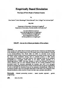
IV. E XPERIMENTAL R ESULT We applied our algorithms to the verification of two XIO devices [8] developed by Rambus Inc. The XIO cell is a highperformance, low-latency controller interface to XDR DRAM memory devices. The verification platform used in this project is specman. Figure 1 shows its architecture. DUT is the device to be verified, which is the XIO device in this paper. The transaction generator generates transactions based on the test constraints and drives inputs to the DUT. The output checker monitors the output signals from DUT and compares them with the correct results from predictor. The coverage data and other information are collected during the simulation by the coverage block.

Checker

Generator

Test

DUT

Coverage Fig. 1.

The Verification Framework

The XIO devices are implemented in the verilog language and simulated by Cadence’s nc-sim simulator. The test cases are coded with the e language. And the vManager tool is used to collect coverage data required by our algorithms. Our algorithms are implemented in the Matlab platform which has the advantage of fast prototyping and powerful visualization. The result of offline algorithms are described first, with the comparison with the result from vManager. Then several methods are used for the online problems and their results are compared. A. Result of Offline Algorithms We apply both the greedy algorithm and relaxed LP based method to the Toshiba XIO device. Figure 2 shows result, where the horizontal axis is for the verification time and the vertical axis indicates the coverage.

super-optimal one at the beginning, we do not think the superoptimal solution is feasible because the integer constraint of Equation 4f is seriously violated. Therefore, there is little benefit to solving the expensive ILP to compute the exact optimal result. From the greedy algorithm’s result, we can see that 169 over 222 test cases are redundant thus can be removed without reducing coverage, or more than 85% time can be saved using the execution order from greedy algorithm. It should be mentioned that the coverage increases to 40% rapidly within 2% of total verification time, which is very useful when there is not enough time to run all test cases to achieve a coverage of 50%. vManager also provides a ranking function to rank the importance of all test cases. We compare the results from vManager and our greedy algorithm. As shown in Figure 3, it is obviously that the results from vManager and greedy algorithm are almost the same. Thus we believe vManager also uses a similar greedy algorithm.

0.5

0.45

Coverage

Predictor

0.4

0.35 default order greedy algorithm vManager

0.5

0.3 0

0.5

1

1.5

2

Time (second)

2.5

3

3.5 5

x 10

0.4

Coverage

Fig. 3.

Result from vManager

0.3

B. Result of Online Algorithms 0.2 default order greedy algorithm sup−optimal(time) sup−optimal(cov)

0.1

0 0

0.5

1

1.5

2

2.5

Time (second) Fig. 2.

3

3.5 5

x 10

Result of Offline Algorithms

In the figure, we noticed that the result from greedy algorithm is much better than the default order and is quite close to the super-optimal order by solving relaxed LP. Although there is a large gap between approximated solution and the

Then the online algorithm is applied to a similar BE-XIO device. To check the efficiency of our algorithm, several other orders are also considered. The default order maintained by engineers lists all test cases mainly by its creation time. The column first order puts all test cases with the same configuration together, and the row first order puts all test cases with the same feature together. The random order select the next test case to execute randomly. The results for these execution order are shown in Figure 4. Obviously, the result for the default order, shown as the black curve in the plot, is the worst one. The column first order and row first order are a little better. And the column first order is usually better than the row first order, which indicates that the similarity of test cases with same feature is usually larger. The blue curve in the plot shows the average result for

0.35

Coverage

0.3

0.25

0.2 default order greedy algorithm column first row first random online

0.15

0.1 0

1

2

3

4

5

Time (second) Fig. 4.

6

7 4

x 10

Result of Online Algorithms

random order, which is slightly better than column first order at the beginning. But there is still big gap between random order and the near optimal order from greedy algorithm. The online algorithm as shown in algorithm 2 produces better result than all other pre-defined orders. However, its result is close to the result from random order at the beginning when the algorithm does not have enough data to predict the importance of a test case accurately. Similarly, the results are similar at the end which can be explained by the large accumulated estimation error in Equation 7. V. C ONCLUSION

AND

F UTURE W ORK

In summary, we improved the performance of simulation based verification by reordering the test cases. We developed both offline algorithms and an online algorithm. The greedy algorithm produces a close to optimal execution order and the online algorithm makes the first execution of the testbench more efficient by predicting the coverage vector and running time of a test case. The results from two XIO devices demonstrate that our algorithms can save large percentage of time for practical verification. The methods presented in this paper are general and can be applied to other AMS circuits as well. First, the offline algorithms can be applied to any verification problem given the precomputed coverage information. Second, the online algorithm can be extended to support similar problems in other

projects. Of course, different methods to predict coverage vectors are required for other testbenches with different structures. Further improvement can be gained by applying similar algorithm to small granularity given it works for large granularity. The testbench is composed of test cases, similarly, a test case usually consists of several components. Optimizing within a test case would be more powerful and reduce more redundancy. However, the reordering method does not work directly for components because they are not independent with each other as are test cases. On the other hand, the coverage of a test case depends on both the order of components and their combinations. This also provides the opportunity to generate new test cases and increase coverage automatically by combining components from different user provided test cases. Of course, it is challenging to handle the dependency between components and generate functionally correct test cases. The online algorithm can be also extended to small granularity. The components in a test case usually have multiple operation modes, for example, there are several different ways to initialize the XIO device. However, it is usually impossible to check all possible cases because the number of combinational cases is huge especially for large circuit. Therefore, only a small subset of typical cases are considered due to time constraints. Now the subset is usually selected manually or randomly which can not guarantee a good result. The online algorithm can be extended to solve the problem because it does not require any information of test cases and produces a close to optimal result automatically. ACKNOWLEDGMENT We would like to thank Mark Greenstreet for his advice on the mathematical model, and also thank Kathryn Mossawir, Tom Sheffler, John Hong and Victor Konrad for their help on this project. R EFERENCES [1] K. Thomas, Introduction to Formal Hardware Verification. Springer, 1999. [2] E. M. Clarke and B.-H. Schlingloff, Model checking. Amsterdam, The Netherlands, The Netherlands: Elsevier Science Publishers B. V., 2001. [3] K. L. McMillan, Symbolic Model Checking. Norwell, MA, USA: Kluwer Academic Publishers, 1993. [4] N. Metropolis and S. Ulam, “The monte carlo method,” Journal of the American Statistical Association, vol. 44, no. 247, pp. 335–341, 1949. [5] A. Schrijver, Theory of linear and integer programming. New York, NY, USA: John Wiley & Sons, Inc., 1986. [6] N. Jorge and W. Stephen, Numerical Optimization. Springer, 2000. [7] “Using the cplex linear optimizer,” CPLEX Optimization Inc, Incline Village, NV, 1994. [8] “Xdr io cell technical document.” [Online]. Available: http://www.rambus.com/us/downloads/document abstracts/products/dl 0362 v0 71.html