demanda entre els cientıfics que estudien els diferents aspectes del fons sub- ...... [36] R. M. Eustice, H. Singh, J. J Leonard, and M. R Walter. Visu- ally mapping ...
EFFICIENT TOPOLOGY ESTIMATION FOR LARGE SCALE OPTICAL MAPPING
Armagan ELIBOL
Dipòsit legal: GI-1322-2011 http://hdl.handle.net/10803/41944
ADVERTIMENT. La consulta d’aquesta tesi queda condicionada a l’acceptació de les següents condicions d'ús: La difusió d’aquesta tesi per mitjà del servei TDX ha estat autoritzada pels titulars dels drets de propietat intel·lectual únicament per a usos privats emmarcats en activitats d’investigació i docència. No s’autoritza la seva reproducció amb finalitats de lucre ni la seva difusió i posada a disposició des d’un lloc aliè al servei TDX. No s’autoritza la presentació del seu contingut en una finestra o marc aliè a TDX (framing). Aquesta reserva de drets afecta tant al resum de presentació de la tesi com als seus continguts. En la utilització o cita de parts de la tesi és obligat indicar el nom de la persona autora. ADVERTENCIA. La consulta de esta tesis queda condicionada a la aceptación de las siguientes condiciones de uso: La difusión de esta tesis por medio del servicio TDR ha sido autorizada por los titulares de los derechos de propiedad intelectual únicamente para usos privados enmarcados en actividades de investigación y docencia. No se autoriza su reproducción con finalidades de lucro ni su difusión y puesta a disposición desde un sitio ajeno al servicio TDR. No se autoriza la presentación de su contenido en una ventana o marco ajeno a TDR (framing). Esta reserva de derechos afecta tanto al resumen de presentación de la tesis como a sus contenidos. En la utilización o cita de partes de la tesis es obligado indicar el nombre de la persona autora. WARNING. On having consulted this thesis you’re accepting the following use conditions: Spreading this thesis by the TDX service has been authorized by the titular of the intellectual property rights only for private uses placed in investigation and teaching activities. Reproduction with lucrative aims is not authorized neither its spreading and availability from a site foreign to the TDX service. Introducing its content in a window or frame foreign to the TDX service is not authorized (framing). This rights affect to the presentation summary of the thesis as well as to its contents. In the using or citation of parts of the thesis it’s obliged to indicate the name of the author.
PhD Thesis
Efficient Topology Estimation for Large Scale Optical Mapping
Armagan Elibol
2011
Doctoral Programme in Technology
Supervised by: Rafael Garcia and Nuno Gracias
Work submitted to the University of Girona in fulfilment of the requirements for the degree of Doctor of Philosophy.
We, Rafael Garcia and Nuno Gracias, senior researchers of the Institute of Informatics and Applications at the University of Girona
ATTEST: that this thesis, titled “Efficient Topology Estimation for Large Scale Optical Mapping”and submitted by Armagan Elibol for the degree of Ph.D. in Technology, was carried out under our supervision. Signed:
Dr. Rafael Garcia
Dr. Nuno Gracias
Abstract Large scale image mosaicing methods are in great demand among scientists who study different aspects of the seabed, and have been fostered by impressive advances in the capabilities of underwater robots in gathering optical data from the seafloor. Cost and weight constraints mean that low-cost Remotely operated vehicles (ROVs) usually have a very limited number of sensors. When a low-cost robot carries out a seafloor survey using a downlooking camera, it usually follows a predefined trajectory that provides several non time-consecutive overlapping image pairs. Finding these pairs (a process known as topology estimation) is indispensable to obtaining globally consistent mosaics and accurate trajectory estimates, which are necessary for a global view of the surveyed area, especially when optical sensors are the only data source. This thesis presents a set of consistent methods aimed at creating large area image mosaics from optical data obtained during surveys with low-cost underwater vehicles. First, a global alignment method developed within a Feature-based image mosaicing (FIM) framework, where nonlinear minimisation is substituted by two linear steps, is discussed. Then, a simple four-point mosaic rectifying method is proposed to reduce distortions that might occur due to lens distortions, error accumulation and the difficulties of optical imaging in an underwater medium. The topology estimation problem is addressed by means of an augmented state and extended Kalman filter combined framework, aimed at minimising the total number of matching attempts and simultaneously obtaining the best possible trajectory. Potential image pairs are predicted by taking into 3
account the uncertainty in the trajectory. The contribution of matching an image pair is investigated using information theory principles. Lastly, a different solution to the topology estimation problem is proposed in a bundle adjustment framework. Innovative aspects include the use of fast image similarity criterion combined with a Minimum spanning tree (MST) solution, to obtain a tentative topology. This topology is improved by attempting image matching with the pairs for which there is the most overlap evidence. Unlike previous approaches for large-area mosaicing, our framework is able to deal naturally with cases where time-consecutive images cannot be matched successfully, such as completely unordered sets. Finally, the efficiency of the proposed methods is discussed and a comparison made with other state-of-the-art approaches, using a series of challenging datasets in underwater scenarios.
Resum Els m`etodes de generaci´o de mosaics de gran escala gaudeixen d’una gran demanda entre els cient´ıfics que estudien els diferents aspectes del fons submar´ı, afavorida pels impressionants aven¸cos en les capacitats dels robots submarins per a l’obtenci´o de dades ptiques del fons. El cost i el pes constitueixen restriccions que impliquen que els vehicles operats remotament disposin habitualment d’un nombre limitat de sensors. Quan un robot de baix cost du a terme una exploraci´o del fons submar´ı utilitzant una c`amera apuntant cap al terreny, aquest segueix habitualment una traject`oria que d´ona com a resultat diverses parelles d’imatges amd superposici´o de manera sequencial. Trobar aquestes parelles (estimaci´o de la topologia) ´es una tasca indispensable per a l’obtenci´o de mosaics globalment consistents aix´ı com una estimaci´o de traject`oria precisa, necess`aria per disposar d’una visi´o global de la regi´o explorada, especialment en el cas en qu`e els sensors `optics constitueixen l’´ unica font de dades. Aquesta tesi presenta un conjunt de m`etodes robustos destinats a la creaci´o de mosaics d’`arees de grans dimensions a partir de dades `optiques (imatges) obtingudes durant exploracions realitzades amb vehicles submarins de baix cost. En primer lloc, es presenta un m`etode d’alineament global desenvolupat en el context de la generaci´o de mosaics basat en caracter´ıstiques 2D, substituint una minimitzaci´o no lineal per dues etapes lineals. Aix mateix, es proposa un m`etode simple de rectificaci´o de mosaics basat en quatre punts per tal de reduir les distorsions que poden apar`eixer a causa de la distorsi´o de les lents, l’acumulaci´o d’errors i les dificultats d’adquisici´o d’imatges en el medi submar´ı. 5
El problema de l’estimaci´o de la topologia s’aborda mitjanant la combinaci´o d’un estat augmentat amb un filtre de Kalman est`es, amb l’objectiu de minimitzar el nombre total d’intents de cerca de correspond`encies i obtenir simult`aniament la millor traject`oria possible. La predicci´o de les parelles d’imatges potencials t´e en compte la incertesa de la traject`oria, i la contribuci´o de l’obtenci´o de correspond`encies per a un parell d’imatges s’estudia d’acord amb principis de la teoria de la informaci´o. Aix´ı mateix, el problema de l’estimaci´o de la topologia ´es abordat en el context d’un alineament global. Les innovacions inclouen l’´ us d’un criteri r`apid per a determinaci´o de la similitud entre imatges combinat amb una soluci´o basada en arbres d’expansi´o m´ınima, per tal d’obtenir una topologia provisional. Aquesta topologia ´es millorada mitjanant l’intent de cerca de correspond`encies entre parelles d’imatges amb major probabilitat de superposici´o. Contr`ariament al que succe¨ıa en solucions pr`evies per a la construcci´o de mosaics de grans `arees, el nostre entorn de treball ´es capa¸c de tractar amb casos en qu`e imatges consecutives en el temps no han pogut ser relacionades satisfact`oriament, com ´es el cas de conjunts d’imatges totalment desordenats. Finalment, es discuteix l’efici`encia del m`etode proposat i es compara amb altres solucions de l’estat de l’art, utilitzant una s`erie de conjunts de dades complexos en escenaris subaqu`atics.
...to my parents and my brother.
Acknowledgements First of all, I must start by stating that there are no words sufficient to express my gratitude to my supervisors, Rafa and Nuno, who are the best people to work with. I owe much to their endless patience, willingness to work, encouragement, enthusiasm, support, understanding and positive attitude. I am very grateful to all my friends in the Underwater Vision Lab for their tremendous support, great friendship and unlimited help: Olivier, whose help and support made it possible to overcome numerous problems; Tudor, who showed me over several weekends how the lab can be a fun place to work; Ricard, who showed how much one could be against change and at the same time a very good friend of a newly incorporated foreign PhD student; Jordi, whose difficult questions and constructive discussions about maths have helped me to realise how to apply theory to real life; Birgit, Quintana, Laszlo, Ricard Campos and all the others. I have spent the best years of my life with you, and really appreciate everything you have done for me. Thanks a lot. I wish to express my appreciation also to the all members of VICOROB for being very welcoming and kind to me: Xavier Cuf´ı, Joan Mart´ı, Jordi Freixenet, Pere Ridao, Arnau Oliver, Xavier Llad´o, and all the others who were always ready to help from the day I first arrived in Girona. I am also grateful to the secretaries, Anna and Rosa, who were always willing to help me understand paperwork. I am thankful to my flatmate, Carles who is not only a great friend but also a creative chef, and his parents who made me feel very comfortable. I would like to thank David Adamson and his family for helping me greatly to get used to living abroad. I also wish to thank Peter 9
Redmond for his invaluable inputs into the improvement of my English skills. Thanks also to my dear friends, Fatma and Ulku, who were always with me and provided a great amount of support from a distance, in Turkey. Finally, my special thanks go to my parents and my brother, who have given their unconditional support and have always believed in me. To them I dedicate this thesis.
Contents Table of Contents
i
1 Introduction
1
1.1
Objectives . . . . . . . . . . . . . . . . . . . . . . . . . . . . .
4
1.2
Outline of the approach . . . . . . . . . . . . . . . . . . . . .
4
1.3
Contributions . . . . . . . . . . . . . . . . . . . . . . . . . . .
6
1.4
Thesis structure . . . . . . . . . . . . . . . . . . . . . . . . . .
8
2 Feature-Based Image Mosaicing 2.1
2.2
Feature based pairwise image alignment
11 . . . . . . . . . . . . 11
2.1.1
Planar motion models . . . . . . . . . . . . . . . . . . 13
2.1.2
Homography estimation methods . . . . . . . . . . . . 18
Global alignment . . . . . . . . . . . . . . . . . . . . . . . . . 22 2.2.1
Review of global alignment methods . . . . . . . . . . 24
3 New Global Alignment Method
31
3.1
Iterative global alignment . . . . . . . . . . . . . . . . . . . . 31
3.2
Reducing image size distortions . . . . . . . . . . . . . . . . . 35
3.3
Experimental results . . . . . . . . . . . . . . . . . . . . . . . 36
3.4
Chapter summary . . . . . . . . . . . . . . . . . . . . . . . . . 47
4 Combined ASKF-EKF Framework for Topology Estimation 51 4.1
Introduction . . . . . . . . . . . . . . . . . . . . . . . . . . . . 52
4.2
Kalman filter based image mosaicing approaches . . . . . . . . 52 i
4.3 Efficient closed-form solution for calculating the observation mutual information . . . . . . . . . . . . . . . . . . . . . . . . 56 4.4 ASKF-EKF combined framework for topology estimation . . . 58 4.4.1 Definitions . . . . . . . . . . . . . . . . . . . . . . . . . 59 4.4.2 Implementation . . . . . . . . . . . . . . . . . . . . . . 61 4.5 Experimental results . . . . . . . . . . . . . . . . . . . . . . . 66 4.6 Chapter summary . . . . . . . . . . . . . . . . . . . . . . . . . 75 5 Topology Estimation using Bundle Adjustment 77 5.1 Topology estimation using bundle adjustment . . . . . . . . . 79 5.1.1 Model definitions and nomenclature . . . . . . . . . . 79 5.1.2 5.1.3 5.1.4
Initialisation . . . . . . . . . . . . . . . . . . . . . . . . 80 Finding potential overlapping image pairs . . . . . . . 82 Selection and image matching . . . . . . . . . . . . . . 83
5.1.5 5.1.6
Minimising the reprojection error . . . . . . . . . . . . 84 Uncertainty propagation . . . . . . . . . . . . . . . . . 86
5.1.7 Dealing with broken trajectories . . . . . . . . . . . . . 88 5.2 Experimental results . . . . . . . . . . . . . . . . . . . . . . . 89 5.3 Chapter summary . . . . . . . . . . . . . . . . . . . . . . . . . 96 6 Conclusions
99
6.1 Summary . . . . . . . . . . . . . . . . . . . . . . . . . . . . . 99 6.2 Resulting Publications . . . . . . . . . . . . . . . . . . . . . . 100 6.3 Directions for future work . . . . . . . . . . . . . . . . . . . . 101
ii
List of Figures 1.1
Photometric underwater artefacts . . . . . . . . . . . . . . . .
2
1.2
Snapshot of the Unmanned underwater robot (UUR) GARBI .
6
1.3
Snapshot of the Unmanned underwater robot (UUR) ICTINEU
7
2.1
Pipeline of FIM . . . . . . . . . . . . . . . . . . . . . . . . . . 13
2.2
Degrees of freedom of the planar projective transformation . . 16
2.3
Example of error accumulation from registration of sequential images . . . . . . . . . . . . . . . . . . . . . . . . . . . . . . . 23
3.1
Capel’s and the iterative method comparative examples . . . . 33
3.2
Corners of the Euclidean mosaic . . . . . . . . . . . . . . . . . 37
3.3
Corners of the projective mosaic . . . . . . . . . . . . . . . . . 38
3.4
Final mosaic after applying four point homography . . . . . . 38
3.5
Snapshot of the ICTINEU Unmanned underwater robot (UUR) 39
3.6
Uncertainties of the initial estimation . . . . . . . . . . . . . . 40
3.7
Reprojection error vs. iterations . . . . . . . . . . . . . . . . . 41
3.8
Resulting mosaics of the first dataset . . . . . . . . . . . . . . 42
3.9
Resulting mosaics of the second dataset . . . . . . . . . . . . . 45
3.10 Radial distortion was partially compensated. . . . . . . . . . . 46 3.11 Initial estimation and number of tracked features of the underwater sequence . . . . . . . . . . . . . . . . . . . . . . . . . 47 3.12 Resulting mosaics of the underwater image sequence and ground truth mosaic obtained by registering each image to the poster. . . . . . . . . . . . . . . . . . . . . . . . . . . . . . 48 iii
3.13 Solid (red) line shows the ground truth trajectory obtained by registering individual images to the image of the poster. Dashed (green) line denotes the trajectory obtained by the proposed method while the dotted (blue) line shows the trajectory of Capel’s Method. Top left corner of the first image is chosen as an origin of the mosaic frame. . . . . . . . . . . . 49 4.1 Pipeline of the proposed framework . . . . . . . . . . . . . . . 62 4.2 Computing overlapping pairs . . . . . . . . . . . . . . . . . . . 65 4.3 Image vectors with uncertainty convolution . . . . . . . . . . . 65 4.4 Final trajectory of the first dataset. . . . . . . . . . . . . . . . 68 4.5 Overlapping image pairs of the first dataset . . . . . . . . . . 68 4.6 Final mosaic of the first dataset . . . . . . . . . . . . . . . . . 69 4.7 Final topology of the second dataset . . . . . . . . . . . . . . 71 4.8 Final topology of the third dataset . . . . . . . . . . . . . . . 73 4.9 Final topology of the fourth dataset . . . . . . . . . . . . . . . 74 5.1 Pipeline of the proposed scheme . . . . . . . . . . . . . . . . . 79 5.2 Initial similarity matrix of the first dataset. . . . . . . . . . . . 89 5.3 Final trajectory and its uncertainty of the first dataset . . . . 91 5.4 Initial similarity matrix of the second dataset. . . . . . . . . . 92 5.5 Final trajectory and its uncertainty of the second dataset . . . 93 5.6 Initial similarity matrix of the third dataset. . . . . . . . . . . 94 5.7 Final trajectory and its uncertainty of the third dataset . . . . 95 5.8 Initial similarity matrix of the last dataset . . . . . . . . . . . 96 5.9 Final trajectory and its uncertainty of the last dataset . . . . 98
iv
List of Tables 3.1 3.2
Four-point warping algorithm. . . . . . . . . . . . . . . . . . . 37 Characteristics of the datasets. . . . . . . . . . . . . . . . . . 40
3.3 3.4
Results of the tested methods. . . . . . . . . . . . . . . . . . 43 Distortion measures of the final mosaics for the second dataset. 44
4.1
ASKF step . . . . . . . . . . . . . . . . . . . . . . . . . . . . . 63
4.2 4.3
Summary of results for the first dataset. . . . . . . . . . . . . 67 Summary of results for the second dataset. . . . . . . . . . . . 71
4.4 4.5
Comparison of expected overlap and combined strategy . . . . 72 Summary of results for the fourth dataset. . . . . . . . . . . . 74
5.1
Summary of results for the first dataset. . . . . . . . . . . . . 90
5.2 5.3
Summary of results for the second dataset. . . . . . . . . . . . 91 Summary of results for the third dataset. . . . . . . . . . . . . 94
5.4
Summary of results for the last dataset. . . . . . . . . . . . . . 95
v
List of Acronyms SIFT Scale invariant feature transform SURF Speeded up robust features RANSAC Random sample consensus LMedS Least median of square SLAM Simultaneous localisation and mapping DOF Degree of freedom SSD Sum of squared differences DVL Doppler velocity log INS Inertial navigation system USBL Ultra short base line ROV Remotely operated vehicle AUV Autonomous underwater vehicle DLT Direct linear transformation SVD Singular value decomposition KF Kalman filter ASKF Augmented state Kalman filter EKF Extended Kalman filter IEKF Iterated extended Kalman filter BA Bundle adjustment FIM Feature-based image mosaicing OMI Observation mutual information vii
UUV Unmanned underwater vehicle UUR Unmanned underwater robot UV Underwater vehicle UAV Unmanned aerial vehicle MST Minimum spanning tree
viii
Chapter 1 Introduction Over the last two decades, Underwater vehicles (UVs) have greatly improved as a tool for undersea exploration and navigation. In particular, autonomous navigation, localisation and mapping through optical imaging have become topics of great interest for both researchers in underwater robotics and marine science. When UVs perform missions near the seafloor, optical sensors can be used for several different purposes such as obstacle avoidance, motion planning, localisation and mapping. These sensors are especially useful in the case of low-cost robots, which incorporate a very limited sensor suite. The pose (position and orientation) of a low-cost underwater robot can be calculated by integrating the apparent motion between consecutive images acquired by a down-looking camera carried by the vehicle. Knowledge of the pose at image acquisition instances can also be used to align consecutive images to form a mosaic, i.e., a composite image which covers the entire area imaged by the submersible. Several strategies in the literature have attempted to recover vehicle motion using visual mosaics [45, 108, 7]. Once the map has been constructed, the mosaic serves several purposes, such as: 1. To carry out map-based navigation, planning the path of the vehicle during the execution of the mission; 2. To serve as a high-resolution image to perform further processing such as localising interest areas, planning operations on the seafloor and 1
enabling the detection of temporal changes in marine habitats. Underwater images are becoming crucial for studying the ocean, and especially in the understanding of biological and geological processes happening on the seafloor. The characteristics of an underwater environment are very challenging for optical imaging, mainly due to the significant attenuation and scattering of visible light [87, 68]. Commonly, underwater images suffer from lack of contrast, blurring, and variable illumination due to refracted sunlight or artificial illumination (see Figs. 1.1) Moreover, light attenuation does not allow images to be taken from a long distance. Therefore, mosaicing techniques are needed to create high-resolution maps of the surveyed area using a large number of acquired images and to get a global perspective of the underwater terrain [45, 89, 109, 60, 94, 96]. Thus, robotic exploration with the aim of constructing photo-mosaics is becoming a common requirement in geological [112, 33] and archaeological surveys [36], mapping [59], ecology studies [56, 66, 89], environmental damage assessment [41, 65] and temporal change detection [29]. Owing to the rapid development in data
(a)
(b)
(c)
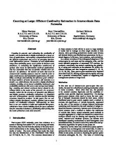
Figure 1.1: Photometric underwater artefacts: (a) Artefacts such as sun flicker, cast shadows, suspended particles, moving plants and fishes that appear in shallow water; (b) Artefacts such as blur, scattering and non uniform illumination that appear in a water column due to artificial lighting, high turbidity and floating life forms; (c) Artefacts such as loss of colour and lack of contrast that appear in deep water.
acquisition platforms, there is an increasing need for large-scale image mosaicing methods. When the mosaic is later used for localisation of interest areas and temporal change detection, the quality constraints for building image mosaics can be very strict. Hence, highly accurate image registration 2
methods are necessary. Although recent advances in the detection of correspondences between overlapping images have resulted in very effective image registration methods [71, 11], all images have to be represented in a common (mosaic) frame in order to obtain a global view of the surveyed area. This process is known as global alignment or global registration. Mostly, global alignment is the process of nonlinear minimisation of a predefined error term [105, 23, 73, 38], and involves a high computational cost for building large area mosaics. Generally, when lacking other sensor data (e.g., Ultra short base line (USBL), Doppler velocity log (DVL), gyrocompass), time-consecutive images are assumed to have an overlapping area. This overlap allows the images to be registered and an initial estimate of the camera trajectory to be obtained over time. This initial dead-reckoning estimate suffers from a rapid accumulation of registration errors, leading to drifts from the real trajectory, but it does provide useful information for the detection of non time-consecutive overlapping images. Matching non time-consecutive images is a key step in refining the trajectory followed by the robot using global alignment methods [105, 98, 23, 43, 38, 30]. With the refined trajectory, new non timeconsecutive overlapping images can be predicted and attempted to match. The iterative matching and optimisation process continues until no new overlapping images are detected. This process is known as topology estimation. In the context of this thesis, we refer to topology estimation as the problem of finding overlapping image pairs among different transect(s) of the surveyed area. Finding matches among non time-consecutive image pairs is usually referred to as loop-closing, i.e., detecting that the area being explored has been visited before. Closing loops is essential to reduce the uncertainty of the trajectory estimation [13, 25, 26, 53, 54, 57, 37]. Impressive progress has recently been achieved in the field of Simultaneous localisation and mapping (SLAM) for underwater platforms equipped with either cameras [74, 101, 36] or sonars [85, 95, 92]. SLAM approaches are well suited to navigation applications such as real-time control and localisation of vehicles, and have been successfully used for online image mosaicing in medium-sized data sets [40, 94]. 3
This contrasts with offline batch approaches, where the data is processed a posteriori. By avoiding real-time constraints, large-scale optimisation methods can be used with considerably larger data sets and significantly higher accuracy in the final results [33].
1.1
Objectives
The scope of this thesis encompasses mission scenarios where a low-cost Unmanned underwater vehicle (UUV) is required to map an area of interest (e.g., Figs. 1.2 and 1.3). Many scientifically interesting sites are located in areas which are nearly flat, such as the coral reefs in the Florida Reef Tract [66]. We consider in this thesis cases where the 3D relief of the scene is negligible compared to the altitude of the robot, and the seafloor is therefore assumed to be and is modelled as a planar scene1 . Commonly, low-cost UURs are tele-operated from a mother vessel, and only equipped with a video camera to provide a feedback to the pilot. Although Autonomous underwater vehicles (AUVs) are normally equipped with different sensors such as DVL, Inertial navigation system (INS), USBL and ring laser gyroscopes, most commercially available low-cost ROVs are limited to a video camera, lights, a depth sensor [2, 1], and in some cases a compass [5, 4, 3]. In this thesis, we focus on developing consistent and flexible methods to enable the building of 2D maps of large areas without any additional sensor information apart from that coming from optical sensors, as this is the case for most available UURs. Nonetheless, should additional positioning information available, we also address the topic of fusing such information a naturally integrated way.
1.2
Outline of the approach
Rapid developments in the robotics field have made it possible to collect optical data from places where humans cannot reach. In robot mapping 1
Although the seafloor is seldom totally flat, we use robust estimation methods in this thesis that allow us to deal with moderate levels of 3D content provided that the scene is
4
applications (both aerial and underwater), when a robot is surveying a large area using only a down-looking camera, the aim is to obtain a global view of the area. To obtain a wide-area visual representation of the scene, it is necessary to create large-area optical maps, known as mosaics. When creating large-area mosaics from optical data alone, two main problems need to be addressed: global alignment and topology estimation. Global alignment refers to finding the registration parameters between each image and the chosen global frame, while topology estimation refers to detecting overlapping image pairs and creating a graph linking the overlapping images that can be matched. Much of the research effort that has gone into this thesis has focused on the global alignment and topology estimation parts of the FIM framework. An iterative linear solution in the mosaic frame is presented for the global alignment problem. While working in the mosaic frame, some distortions might appear in the image size. To deal with this possibility and to reduce its effects on the final mosaic, a simple but efficient four-point mosaic rectifying algorithm is proposed. This algorithm can also be seen as a fast way to fuse any additional sensor information whenever it is available. Secondly, two different frameworks, Kalman filter (KF) and Bundle adjustment (BA), are described and detailed for the topology estimation problem. They are both aimed at getting the best possible globally coherent mosaic and trajectory estimate with the minimum number of image matching attempts by exploring the contributions of matching different image pairs, and deciding which image pairs should be matched first. The KF framework opens the door to a new way of using existing theories for control and estimation problems in the context of batch mosaicing. The image acquisition process in large area surveys often takes several days due to limitations of UURs such as power, sensor coverage and camera field of view, and the difficulties introduced by underwater medium such as light absorption, scattering and back scattering. As a result, time-consecutive images do not necessarily always have an overlapping area. Also, UURs sometimes move too fast, causing motion blur between overlapping images and predominantly planar.
5
Figure 1.2: Snapshot of the UUR GARBI [6] operating in the test pool of the University of Girona.
pairwise image registration to fail. To be able to estimate the topology where there could be gaps between time-consecutive images, a BA based topology estimation framework is proposed. This framework first tries to infer a possible topology using an image similarity measure based on the similarity of feature descriptors. It then makes use of one of the well-known graph theory algorithms, MST, to establish links between images. A weighted reprojection error is minimised over the trajectory parameters and its uncertainty calculated using first order propagation [50]. New possible overlapping image pairs are predicted by taking into account the trajectory uncertainty.
1.3
Contributions
The main contributions of this thesis can be summarised as follows: • A novel global alignment method is proposed. This method works in the global frame and uses two linear steps iteratively to obtain globally coherent mosaics. It is faster and does not require as much computational effort and memory as its counterparts. 6
Figure 1.3: Snapshot of the UUR ICTINEU [93] operating in the Mediterranean Sea.
• Kalman filter formulations are adapted to address the topology estimation problem of creating large area mosaics. The presence of overlap between an image pair is modelled as an observation from a sensor. Different ranking criteria are proposed for rating potential observations, and the problem of finding non time-consecutive images of the surveyed area is formulated as one of sensor selection problem. A novel way of finding overlapping image pairs is proposed, which takes into account position uncertainty. A computationally efficient closed form for calculating Mutual Information is presented as a whole. The proposed framework allows for the use of existing theory for estimation and control problems in the batch mosaicing of large areas, with the aim of reducing the total number of image matching attempts. • The topology estimation problem is addressed in a BA framework and 7
an end-to-end solution for creating large area mosaics is presented. Initial similarity information is obtained from images in a fast way and an efficient use of the information obtained is proposed, based on MST. Closed form equations for the first order uncertainty propagation of the weighted reprojection error are presented. The proposed framework is able to deal with cases where there are gaps between time-consecutive images, such as completely unordered image sets.
1.4
Thesis structure
The thesis is divided into the following chapters. Chapter 2 overviews the FIM framework. Related work on planar motion estimation and global alignment methods is mentioned and the notation used in the thesis is introduced. Chapter 3 details the proposed global alignment method for creating 2D image mosaics. This new method works in the mosaic frame and does not require any non-linear optimisation. The proposed method has been tested with several image sequences and comparative results are presented to illustrate its performance. Chapter 4 addresses the topology estimation problem for creating largearea mosaics. This chapter presents an Augmented State and Extended Kalman filter (EKF) combined framework to solve the problem of obtaining a 2D photo-mosaic with minimum image matching attempts and simultaneously getting the best possible trajectory estimation. It does this by exploring contributions of the matching of the image pairs to the whole system using some information theory principals. Chapter 5 deals with the topology estimation problem in the BA framework. First, it tries to infer some information about the trajectory by extracting and matching a small number of features. Then it uses MST to initialise the links between images. After image matching, the 8
weighted reprojection error is minimised. As a final step, the uncertainty in the trajectory estimation is propagated and used for generating the potential overlapping image pairs. Chapter 6 presents a summary of contributions and identifies some future research directions.
9
Chapter 2 Feature-Based Image Mosaicing FIM can be divided into two main steps: image spatial alignment, also known in the literature as image registration or motion estimation, and image intensity blending for rendering the final mosaic. The spatial alignment step can be further divided into pairwise and global alignments. Pairwise alignment is used to find the motion between two overlapping images; images have to be mapped onto a common frame, also known as the global frame, in order to obtain globally coherent mosaics. Global alignment refers to as the problem of finding the image registration parameters that best comply with the constraints introduced by the image matching. Global alignment methods are used to compensate for the errors in pairwise registration. Although the alignment between images may be close to perfect, intensity differences do not allow the creation of a seamless mosaic. Image blending methods are needed to deal with the problem of intensity differences between images after they have been aligned. Several methods have been proposed for image blending [24, 62, 91, 114] as well as for mosaicing [104]. Pairwise and global alignment methods are reviewed and detailed later in this chapter.
2.1
Feature based pairwise image alignment
Two dimensional(2D) image alignment is the process of overlaying two or more views of the same scene taken from different viewpoints while assuming 11
that the scene is approximately flat. This overlaying requires an image registration process to determine how the images warp into a common reference frame. Several approaches exist to register these images [113]. The pipeline of feature-based image registration between overlapping images is illustrated in Fig. 2.1. Feature-based registration methods rely on the detection of salient features using Harris [51], Hessian [12] or Laplacian [64] detectors. These features are detected in the two images to be registered, and then a correlation or a Sum of squared differences (SSD) measure is computed around each feature. This was the trend for many years, until the advent of Scale invariant feature transform (SIFT) algorithm proposed by Lowe [70]. The satisfactory results of this method have greatly speeded up the development of salient point detectors and descriptors, and taken feature-based matching techniques to the forefront of research in computer vision. Compared to all formerly proposed schemes, SIFT and subsequently developed methods such as Speeded up robust features (SURF) [11] demonstrate considerably greater invariance to image scaling, rotation and changes in both illumination and the 3D camera viewpoint. These methods solve the correspondence problem through a pipeline that involves (1) feature detection, (2) feature description and (3) descriptor matching. Feature detection is based on either Hessian or Laplacian detectors (the “difference of Gaussians” of SIFT is an approximation of the Laplacian, and SURF uses an approximation of the Hessian). Feature description exploits gradient information at a particular orientation and spatial frequency (see [80] for a detailed survey of descriptors). Finally, the matching of features is based on the Euclidean distance between their descriptors [71], whereby corresponding points are detected in each pair of overlapping images. The initial matching frequently produces incorrect correspondences (due to noise or repetitive patterns, for example) which are called outliers. Outliers should be rejected with a robust estimation algorithm (e.g., Random sample consensus (RANSAC) [39] or Least median of square (LMedS) [79]). These algorithms are used to estimate the dominant image motion which agrees with that of the largest number of points. Outliers are identified as the points that do not follow that dominant motion. After outlier rejec12
Figure 2.1: Pipeline of feature-based image registration between an overlapping image pair
tion, a homography can be computed from the inliers through orthogonal regression [52].
2.1.1
Planar motion models
A homography is the planar projective transformation that relates any two images of the same plane in 3D space and is a linear function of projective image coordinates [103, 52]. The planar homography matrix is able to describe a motion with eight Degree of freedoms (DOFs). For scientific mapping applications, the eight DOFs of the planar homography may contain more DOFs than would be strictly necessary. In these cases, it is possible to set-up constrained homography matrices describing a more reduced set of DOFs (see Figure 2.2). Such a reduced set of DOFs will have the advantages of being less sensitive to noise and, in most cases, being faster to estimate. Let I denote the image taken at time t, and I ′ the image acquired at time t − 1. I ′ and I are two consecutive images of a monocular video sequence which have an overlapping area. In special circumstances1 , it can be assumed that the scene, in our case the seafloor, is planar. Under this assumption the 1
For example, when the 3D relief of the scene is much smaller than the distance from the camera to the scene.
13
homography that relates I ′ and I can be described by the planar transformation p′ = Hp, where p′ denotes the image coordinates of the projection of a 3D point P onto the image plane at time t − 1 and p is the projection of the same 3D point onto the image plane at time t; then p = (x, y, 1)T and p′ = (x′ , y ′, 1)T are called correspondences and expressed in homogeneous coordinates. Homogeneous coordinates of a finite point (x, y) in the plane are defined as a triplet (λx, λy, λ) where λ 6= 0 is an arbitrary real number. Coordinates (x1 , y1 , 0) describe the point at infinity in the direction of slope β = xy11 . Given a corresponding pair of points p = (x, y, 1)T and p′ = (x′ , y ′, 1)T in I and I ′ respectively, the homography H is a 3 × 3 matrix defined up to scale, that satisfies the constraint between both points in accordance with λ′ p′ = Hp, where λ′ is an arbitrary non-zero scaling constant. Some homography estimation methods from multiple correspondences based on Direct linear transformation (DLT) will be summarised later and a detailed review of estimation methods can be seen in [52]. Most commonly used planar transformations can be classified into one of four main groups according to their DOFs, which are the number of parameters that might vary independently. Euclidean. Euclidean transformation has three DOFs, two for translation and one for rotation. This transformation is composed of translation and rotation in the image plane and can be parameterised as;
′
x cos θ − sin θ tx x ′ y = sin θ cos θ ty y 1 0 0 1 1
(2.1)
where θ is the amount of rotation and tx , ty correspond to the translation along the x and y axes. The scale of the objects in the image is not allowed to change. In order to calculate a Euclidean transformation, a minimum of two correspondences are needed, since one correspondence provides two independent constraints on the elements of the homography. This type of transformation is suitable for strictly controlled robot trajectories in which the robot maintains a constant altitude and 14
only a rotation around the optical axis of its camera is allowed. Similarity. A similarity transformation is the generalisation of the Euclidean transformation that allows for scale changes. It has four DOFs, one for rotation, two for translation and one for scaling. Two correspondences are also enough to calculate similarity transformations. It can be expressed as
x′ s cos θ − s sin θ tx x ′ y = s sin θ s cos θ ty y 1 0 0 1 1
(2.2)
where s is the scaling parameter and models the changes in the robot’s altitude. This type of transformation is used to model robot trajectories in which the robot is allowed to change its altitude during the mission. Affine. The affine transformation is more general than the similarity, and has six DOFs. As a result, the minimum number of correspondences to calculate an affine transformation is three;
′
x h h t x 11 12 x y ′ = h21 h22 ty y 1 0 0 1 1
(2.3)
The first four elements of an affine transformation can be decomposed into the product of three rotation matrices and one diagonal matrix, using Singular value decomposition (SVD) [52]: h11 h12 h21 h22
!
! ! cos θ − sin θ cos(−φ) − sin(−φ) = · sin θ cos θ sin(−φ) cos(−φ) ! ! (2.4) cos φ − sin φ ρ1 0 · · 0 ρ2 sin φ cos φ
From Eq. (2.4) it can be seen that affine transformations first apply a rotation by an angle φ, followed by an anisotropic scaling along the 15
(a)
(b)
(c)
(d)
(e)
(f)
Figure 2.2: DOFs of the planar projective transformation on images: (a) horizontal and vertical translations, (b) rotation, (c) scaling, (d) shear, (e) aspect ratio and (f) projective distortion along the horizontal and vertical image axis.
rotated x and y directions, then a back rotation by −φ and finally a rotation by θ. This type of transformation is used to approximate projective transformations, especially where the camera is far from the scene and has a small field of view.
Projective. Projective transformations are the last group of planar transformations. They have eight DOFs and at least four correspondences are needed to compute them:
′ ′
λx h h h x 11 12 13 λ′ y ′ = h21 h22 h23 y ′ λ h31 h32 h33 1
(2.5)
where λ′ is an arbitrary scaling factor. The result of Eq. (2.5) is: x′ =
h11 x+h12 y+h13 h31 x+h32 y+h33
y′ =
h21 x+h22 y+h23 h31 x+h32 y+h33
(2.6)
Projective homographies can also be inferred using 3D camera projection matrices and a description of a 3D plane. Correspondences between images are the projection of identical world points onto two images with different camera positions and orientations (pose), or two different cameras. Let the 3D world coordinate frame be the first camera frame. In this case, given a 16
point P in the scene, its projection matrices can be written as:
. p = K[I 0] ′ ′ . ′ ′ p = K [R t ] ′
(2.7)
′
′
where K and K are camera’s intrinsic parameter matrices, R and t describe the rotation and translation between the camera frames, expressed in the . frame of the first camera, and = indicates equality up to scale. A 3D plane that does not contain the optical centres of the cameras can be defined by its normal vector n and perpendicular distance d1 to the optical centre of the first camera. In our case, the underwater robot is moving and taking pictures of the seabed. This means that the intrinsic parameters of the cameras are ′ equal, i.e., K = K in Eq. (2.7). Let p1 and p2 be the coordinates of the ′
image projections of the same 3D point P. The relation between p and p can be written as [72]
′ . ′ ′ T p = K[R + t nd1 ]K−1 p ′ T ′ H = K[R + t nd1 ]K−1
(2.8)
The homography in Eq. (2.8) has six (three translational and three rotational parameters) DOFs assuming that the camera is calibrated. This allows us to represent the projective homography with six instead of eight DOFs like in Eq. (2.5), which can reduce computational cost and improve the accuracy of homography estimation. Moreover, while the robot is executing a trajectory, rotation and translation between consecutive images do not change abruptly due to robot dynamics. This helps to define bounds for the parameters. The bounds are helpful when using nonlinear methods to minimise the cost functions. Since homographies are obtained up to a scaling factor, the world plane distance can be set to one unit along the Z axis. Eq. (2.8) can be written according to the reference camera frame that is chosen as the first
17
camera frame; 1
Hi = K[1 Ri +1 ti nTr ]K−1 1 Hj = K[1 Rj +1 tj nTr ]K−1 i
(2.9)
Hj = K[1 Ri +1 ti nTr ]−1 [1 Rj +1 tj nTr ]K−1
where nr , is the vector normal of the world plane, parameterised by two angles, 1 Ri ,1 Rj , are rotation matrices, and 1 ti and 1 tj are the translation vectors.
2.1.2
Homography estimation methods
The estimation of homographies involves minimising a defined cost function. This minimisation can be linear or non-linear depending on the cost function and also on the type of homography. In the case of projective homographies, if the number of correspondences is four, then the mathematically exact solution for H can be obtained. However, although four correspondences are enough, in practice it is not desirable to compute the motion between images with just four points, due to the presence of noise. Since a homography matrix that satisfies {x′i = Hxi }, i = 1 . . . n does not always exist, for all correspondences in the case of n > 4, an approximate homography can be determined by minimising some error functions on a given set of correspondences. A comprehensive set of definitions of different error (cost) functions can be found in [52]. Given n correspondences x ↔ x′ , h = [h11 , h12 , h13 , h21 , h22 , h23 , h31 , h32 , h33 ]T , Eq. (2.6) can be written in the form Ah = 0: x1 y1 1 0 0 0 −x′1 x1 −x′1 y1 − x′1 h11 0 0 0 0 x1 y1 1 −y1′ x1 −y1′ y1 − y1′ h12 0 .. .. .. . . = . x y 1 0 0 0 −x′ x −x′ y − x′ h 0 n n n n n n n 32 ′ ′ ′ 0 0 0 xn yn 1 −yn xn −yn yn − yn h33 0 (2.10) 18
Eq. (2.10) has more rows than columns if n > 4. The most common approach in the literature is to find the least square solution, h, which minimises the residue vector k Ah k. It is of interest to find a non-zero solution, since h = 0 would trivially minimise k Ah k. Such a non-zero solution can be obtained up to scale. When estimating h, this arbitrary scale needs to be fixed, and is generally done by imposing unit norm, k h k= 1, or fixing one element (e.g., h(3, 3) = 1).
Singular value decomposition The solution for h which minimises k Ah k subject to k h k= 1 is the unit singular vector corresponding to the smallest singular value of A. The SVD can therefore be used to obtain the solution [52]. The SVD of a given matrix Am×n , is written as A = UDVT , where Um×m and Vn×n are orthogonal matrices (UUT = I, VVT = I) and D is a diagonal matrix with non-negative elements. The elements of D, d1 , d2 , ..., dn , are singular values of A: (2.11) k Ah k=k UDVT h k=k DVT h k=k Dz k where z = VT h and k z k= 1 since U and V are norm preserving matrices. Eq. (2.11) is minimised by setting z = (0, 0, 0, . . . 1), as D is a diagonal matrix and its elements are sorted in descending order. Finally, the homography is found by means of the equation h = Vz, which corresponds to the last column of V.
Eigenvalue decomposition The error term k Ah k can be expressed as k Ah k = (Ah)2 = (Ah)T (Ah) = hT AT Ah 19
(2.12)
Taking the derivative of Eq. (2.12) with respect to h and setting it to zero in order to minimise leads to the following equation: 1 0 = (AT A + (AT A)T )h 2
(2.13)
Similarly to the SVD solution above, h should equal the eigenvector of AT A that has an eigenvalue closest to zero. This result is the same as the result obtained using SVD due to the fact that, given a matrix A with SVD decomposition A = UDVT , the columns of V correspond to the eigenvectors of AT A.
Pseudo-Inverse solution The inverse of a matrix exists if the matrix is square and has full rank. The pseudo-inverse of a matrix is the generalisation of its inverse and exists for any m × n matrix. Under the assumptions m > n and that A has rank n, the pseudo-inverse of matrix A in Eq. (2.11) is defined as: A+ = (AT A)−1 AT
(2.14)
If h(3, 3) is fixed at 1, Eq. (2.10) can be rewritten as Am×n h = b where b is equal to the last column of the matrix A. The solution can be found by calculating h = A+ b. The pseudo-inverse of a given matrix Am×n can be calculated easily by using SVD. The SVD of matrix A is denoted as A = UDVT , i.e., (AT A)−1 AT = (VDT UT UDVT )−1 VDT UT = (VT )−1 D−1 (DT )−1 V−1 VDT UT = V(DT D)−1 DT UT = VD+ UT
(2.15)
The pseudo-inverse of a given matrix can be calculated by using Eq. (2.14) or (2.15). Vector h can be found by using the formula h = A+ b = VD+ UT b or h = (AT A)−1 AT b. 20
Nonlinear methods A number of nonlinear methods have been proposed for the estimation of homographies [97, 52, 111, 69]. From Eq. (2.5), using the l2 norm, a cost function e can be expressed as follows: n � X
� h21 xi + h22 yi + h23 2 h11 xi + h12 yi + h13 2 ′ ) + (yi − ) e(h) = (xi − h31 xi + h32 yi + 1 h31 xi + h32 yi + 1 i=1 (2.16) where n is the number of correspondences and h = 1 T h = (h11 , h12 , h13 ) 2 h = (h21 , h22 , h23 )T . Finding the h that minimises e(h) is a h3 = (h31 , h32 , 1)T nonlinear least squares problem and can be solved using iterative methods such as Newton iteration or Levenberg-Marquadt [61, 76]. Eq. (2.16) can be ′
written in a closed form e =k f (h) − x′ k
where f (h) =
T
h1 x T h3 x T h2 x 3T h x
(2.17)
. This nonlinear least squares problem can be solved
iteratively under the assumption of f being locally linear. The first order Taylor expansion of f around the value h0 can be written as: f (h) = f (h0 ) +
∂f (h − h0 ) + rn ∂h
(2.18)
where rn is called the remainder and is calculated as follows: rn =
Z
h
f (n+1) (u)
h0
(x − u)n du n!
(2.19)
∂f Consider J = ∂h as a linear mapping represented by the Jacobian of f with respect to the elements of h. Let ǫ0 be defined by ǫ0 = f (h0 ) − x′ . The
approximation of f at h0 is assumed to be f (h0 + ∆h) = f (h0 ) + J∆h. It is of interest to find a point f (h1 ), with h0 + ∆h, that minimises f (h1 ) − x′ which can be written 21
f (h1 ) − x′ = f (h0 ) + J∆h − x′ = e0 + J∆h The term |e0 + J∆h| needs to be minimised over ∆h, which can be done linearly by using normal equations JT J∆h = −JT e0 ∆h = −J+ e0
(2.20)
and h1 = h0 − J+ e0 . Vector h that minimises Eq. (2.17) can be calculated iteratively hi+1 = hi + ∆hi . For i = 0 an initial estimation h0 must be given to start the iteration. In line with the Levenberg-Marquadt algorithm, Eq. (2.20) is changed into the following form: (JT J + λi I)∆hi = −JT ei
(2.21)
where I is the identity matrix and λi is a scalar that controls both the magnitude and direction of ∆hi . Eq. (2.21) is called an augmented normal equation. Since these are iterative methods, the initial estimation plays an important role in achieving convergence and a local extremum. Nonlinear methods can be used not only for projective homographies but also other types where the elements of the homography are non-linear functions of the parameters (e.g., trigonometric), such as the Euclidean model in Eq. (2.1). In this section, three different linear methods and one non-linear method for one cost function have been summarised. In most cases, linear methods provide quite a good estimation [52], but there are some cases where nonlinear methods are used to refine the result. Non-linear methods improve on the accuracy obtained by linear methods, and deciding which method to use depends on the application, as mosaics can serve different purposes.
2.2
Global alignment
When an underwater platform on which a down-looking camera is deployed revisits a previously surveyed area, it becomes essential to detect and match the non-time consecutive overlapping images in order to close a loop 22
and, thus, improve the trajectory estimation. Let k−1 Hk denote the relative homography between the k th and (k − 1)th image in the sequence. The global projection of image k into the mosaic frame is denoted as 1 Hk and is called an absolute homography 2 . This homography can be calculated by composing the transformations 1 Hk = 1 H2 ·2 H3 · . . . ·k−1 Hk . Unfortunately, the correspondences detected between image pairs are subjected to localisation errors, due to noise or illumination effects. The accuracy of the resulting homography may also be limited by the selected estimation method and departures from the assumed scene planarity. Relative homographies therefore have limited accuracy and computing absolute homographies from them, through a cascade product, results in cumulative error. The estimated trajectory will drift from the true value for long sequences when there is only optical information available, and produce large errors in the positioning of images (see Fig. 2.3). When the trajectory
Figure 2.3: Example of error accumulation from registration of sequential images. The same benthic structures appear in different locations of the mosaic due to error accumulation (trajectory drift).
of the camera provides an overlap between non-consecutive images (a closed2
choosing the first image of a sequence as the global frame means that the coordinate system of the first image is also the coordinate system of the mosaic image.
23
loop trajectory), global alignment techniques can be applied to significantly reduce the drift.
2.2.1
Review of global alignment methods
Several methods have been proposed in the literature to solve the global alignment problem [104]. Global alignment usually requires the minimisation of an error term, which is defined from image correspondences. Global alignment methods can be classified according to the domain where the error term is defined, which is commonly either in the image frame [105, 23, 77, 38] or in the mosaic frame [28, 58, 98, 89, 43, 22]. Davis [28] proposed a global alignment method based on solving sparse linear systems of equations created from relative homographies. He considered a problem in which the camera is only rotating around its optical axis, and there is no translation. The absolute homography can be written as an accumulation of relative homographies. As is common practice, the first frame was chosen as the global frame: 1
Hi =
i Y
j−1
Hj
i≥2
(2.22)
j=2
Any image i in the sequence can be projected to another image space j. Using the absolute homography of image j, image i can also be projected to the global frame: 1 H i =1 H j · j H i (2.23) Here the elements of matrices 1 Hi and 1 Hj are unknown and j Hi is a relative homography. For closed loop sequences, the total number of relative homographies is greater than the total number of images. This over-determined system can be solved by the methods summarised in section 2.1.2, which are simple and easy to implement. However, an adequate parameterisation is not used on these elements to take advantage of the special structure of rotationinduced homography. This leads to over parameterisation which might cause overfitting. 24
Szeliski et al. [100] defined the error function on the image frames as: min
1 H ,1 H ,...,1 H 2 3 N
n XXX k
m
1 m kk xj −1 H−1 k · Hm · xj k2
(2.24)
j=1
where k and m are images that have an overlapping area and n is the total number of correspondences between the images. Minimising Eq. (2.24) by using non-linear least squares has the disadvantage that the gradients with respect to the motion parameters are quite complicated and have to be provided for the chosen minimisation method, e.g., the Levenberg-Marquadt. Sawhney et al. [98] defined an error function based on the mosaic frame instead of the image frames: E1 = 1
min
H2 ,1 H3 ,...,1 HN
n XXX k
m
k1 Hk ·k xj −1 Hm ·m xj k2
(2.25)
j=1
where n is the total number of correspondences and k xj and m xj are the j th correspondence between images k and m that have an overlap area. Eq. (2.25) can be minimised under different constraints. If no constraints are imposed, the minimisation of Eq. (2.25) will result in a solution biased towards the reduction of the image size in the mosaic, since the cost function is lower for smaller image sizes. This is referred to as the scaling effect of a mosaic-based cost function. Sawhney et al. [98] therefore introduced and added another term to Eq. (2.25) in order to control the scaling effects on the image size when it is mapped to the global frame: E2 =
N X
k1 Hi .xtr −1 Hi .xbl − (xtr − xbl )k2 + k1 Hi .xtl −1 Hi .xbr − (xtl − xbr )k2
i=1
(2.26) where xtr , xbl , xtl and xbr denote the coordinates of the top-right, bottom-left, top-left and bottom-right corners of the image. Eq. (2.26) tries to minimise the difference in the diagonal length of both the original and mosaic-projected images. A weight factor was used for this penalty term, which forces all images to share nearly the same diagonal length when they are projected onto 25
�
the global frame or mosaic. Unfortunately, forcing the image size to be equal for all images in the sequence causes alignment problems between images because it violates the minimisation of the distances between correspondences. Therefore, the weight factor has to be chosen appropriately. A fixed value can be chosen for every image in the sequence, or it can be increased incrementally since the error gets incrementally larger for every image due to error accumulation. The final error term is the sum of the two terms E1 and E2 mentioned above: E=
n PP P k
N P
k1 Hk .k xj −1 Hm .m xj k2 +
m j=1
k1 Hi .xtr −1 Hi .xbl − (xtr − xbl )k2 + k1 Hi .xtl −1 Hi .xbr − (xtl − xbr )k2
i=1
�
(2.27) The minimisation of Eq. (2.27) has unaffected DOFs (gauge freedoms) [81] under which different solutions related by a common translation and rotation will have the same minima. In order to deal with this problem, Sawhney et al. [98] added the term |H1 · (0, 0, 1)T | to the error in Eq. (2.27) in order to fix the translation of the first image so that only one solution set is found. Instead of fixing the translation, Gracias et al. [43] fixed one of the image frames as a global mosaic frame and aligned all the images with respect to the coordinate system of the fixed frame. The first image frame is usually chosen as a global frame. This can be also done similarly adding a ground control (fiducial) point in SLAM [9]. Although Sawhney et al. [98] used iterative methods to minimise Eq. (2.27) only using corners of overlapping area, Gracias et al. [43] minimised Eq. (2.25) by linear recursive and batch formulation for the similarity type of homographies by using all correspondences. Eq. (2.27) can be minimised linearly for the first three types of homographies: Euclidean, similarity and affine respectively. However, the scaling effect is not dealt with. In [98], Sawhney et al. also proposed a graph-based representation of closed loop trajectories. Each node of the graph represents the position of one image and the edges connect overlapping images. The initial graph only consists of edges between consecutive frames. New edges (arcs) can be 26
added by measuring the distance between image centres. These edges provide additional information to minimise Eq. (2.27). Absolute homographies are calculated by multiplying relative homographies that have already been found between overlapping pairs. Graph based representation is used to reduce the total number of products by searching for the optimal path while computing absolute homographies through relative homographies [58, 77]. This reduces misregistration errors (drift) and distortion effects. Kang et al. [58] proposed a new solution to the global alignment problem also based on graphs. First, a grid of points is defined on the mosaic image. Each node of the graph has a list of the predefined grid points and each grid point has a list of its correspondences to other nodes or images. The correspondences are calculated by using normalised correlation. The error function is defined as the difference between the intensity level of points in the mosaic and their projection in the different images: E=
X
(Im (p) − Ii (p′ ))2
(2.28)
i
where Im (p) is the gray level of point p in the mosaic and Ii (p′ ) is the intensity of the ith image at the projected position of grid point p with p′ =m Hi · p. This error function is used to find the set of correspondences for every grid point. Global registration of frames is done by searching for the optimal path that connects each frame to the reference frame, which is found by geometric distance and the correlation score between every grid point and its correspondences. After this, the location of grid points is adjusted according to their correspondences. To achieve this goal, a weighted average is applied. Weights are the correlation score of the correspondences. Once the grid points have been adjusted, all the absolute homographies accumulated from relative ones can be updated by an adjustment transformation, in the form of a linear transformation between the refined grid points and their correspondences. In this method the grid points on the mosaic play a key role, and they need to be defined very carefully as every image has to contain at least four. These points should also be uniformly distributed and some of them must lie in the overlapping area between images which limits the 27
applicability of the method. Marzotto et al. [77] proposed a similar solution to the problem. In addition to the overlap measure in [98] which is given in Eq. (2.29), they introduced one more measure as shown in Eq. (2.30): dij =
max(|xi − xj | − |ri − rj |/2) min(ri , rj )
(2.29)
where xi and xj are warped image centres while ri and rj are warped image diameters. This distance must be very small compared to the sum of the arc lengths along the minimum sum path between image i to j in the current graph. The optimal path is found by using β values that are calculated βij =
δij ∆ij
(2.30)
where δij is the overlap measure and ∆ij is the cost of the shortest path between nodes i and j. This cost is calculated from the weights, d, on the edges. Absolute homographies are calculated by accumulating relative homographies through the optimal path. The main advantage of using this method to calculate the optimal path is that the homographies are less affected by accumulation errors. For global alignment the error function is defined over a set of grid points on the mosaic. The error of a grid point xk and the total error are defined as follows Ek =
1 XX kxk − Hi ·i Hj · H−1 j xk k2 n i j
(2.31)
where n is the total number of edges between images that contain grid point xk and Hi , Hj denote absolute homographies. The error function is defined as: min E =
m X
Ei2
(2.32)
i
where m is the total number of grid points. Although this strategy has the advantage of distributing the errors, it has some disadvantages, such as: (1) point locations must be chosen very carefully so that every image and 28
overlapping area has enough grid points to calculate the homography, and (2) since the detected feature points are distributed arbitrarily, they may fall in a textureless area, making it difficult to match them in another image. Capel [23] proposed a method to simultaneously minimise both the homography elements and the position of features on the mosaic image. In this method, the same feature point correspondences need to be identified over all views, which requires feature tracking. Let t xi denote the coordinates of the ith interest point defined on the coordinate system of image t and is the image projection of point m xj , which is called the pre-image point and is also usually projected in different views. All the image points that correspond to the projection of the same pre-image point are called N-view matches. The cost function to be minimised is defined as ε1 =
M X X j=1
tx
kt xi − t Hm · m xj k2
(2.33)
i ∈ηj
where M is the total number of pre-image points, ηj is the set of N-view matches, t Hm is a mosaic-to-image homography3 , and k · k2 is the Euclidean norm. In Eq. (2.33), both the homographies and the pre-image points are unknowns. The total number of unknowns, n, can be calculated as follows: n = nDOF × nview + 2 × npoints
(2.34)
where nDOF corresponds to the DOFs of the homography, nview is the total number of views and npoints is the total number of pre-image points. Eq. (2.33) can be minimised by applying non-linear least square methods. The residues inside the error term ε1 are measured in the image frame, but parameterised with points defined on the mosaic frame. This formulation avoids the image scaling bias that occurs when the residues are measured on the mosaic frame. However, as the dataset gets bigger, the total number of 3
m stands for the mosaic frame. This frame can be one of the image frames or a different arbitrary coordinate frame. In this work, the first image frame has been chosen as the mosaic frame and therefore m is equal to 1. For consistency, m has been used in the notation.
29
unknowns dramatically increases, making it impractical for large datasets of several thousand images. Photogrammetric Bundle adjustment (BA) has been a commonly used technique in computer vision research in recent decades. BA presents the problem of refining a visual reconstruction to produce jointly optimal 3D structure and viewing parameter estimates (camera pose and/or calibration) [107]. In this context, optimal means that the parameter estimates are found by minimising the cost function that quantifies the model fitting error, and that the solution is simultaneously optimal with respect to both structure and camera variations. Mostly BA is defined as minimising the reprojection error between the image correspondences, which is defined as the sum of squares of a large number of nonlinear, real-valued functions. Therefore, the minimisation is achieved using nonlinear least-squares methods explained in Section 2.1.2. For image mosaicing, the key issue is solving the global alignment problem by finding optimal motion parameters, from which absolute homographies can be computed. An application of BA to image mosaicing can be found in [78, 46]. Gracias et al. [46] proposed to minimise a cost function defined as follows: n � � XX i E= ki xk −i Hj ·j xk k2 + kj xk −i H−1 · x k k 2 j
(2.35)
i,j k=1
where n is the total number of matches between images i and j, and homographies are represented as in Eq. (2.9). The total number of unknowns is equal to 6 × (nview − 1) + 2. For this method, the camera intrinsics have to be known, which might not be available and/or possible in deep water surveys. This method makes also use of nonlinear optimisation algorithms that require a high computational effort.
30
Chapter 3 A New Global Alignment Method for Feature Based Image Mosaicing As described in the previous chapter, global alignment requires the nonlinear minimisation of an error term, which is defined from image correspondences. In this chapter, a new global alignment method is presented. It works in the mosaic frame and does not require any non-linear optimisation. The proposed method was tested with different image sequences and comparative results are shown to illustrate its performance.
3.1
Iterative global alignment
The proposal is inspired by Capel’s method [23], which tries to simultaneously estimate both the homographies and the position of features on the mosaic image. The proposal is to transfer ε1 in Eq. (2.33) to the mosaic frame in the following equation: ε2 =
M X X
km xj − m Ht · t xi k2
j=1 t xi ∈ηj
31
(3.1)
where
m
Ht is equal to (t Hm )−1 . As was pointed out in the previous chap-
ter, direct minimisation of the error term in Eq. (3.1) biases the estimation towards small image sizes, since smaller images lead to smaller differences between m xj and m Ht · t xi . If the error term in Eq. (3.1) is analysed, one can observe that minimisation can be divided into two linear sub-problems (sub-steps): First Step The first step is to minimise the error by considering the homography values to be constant, and therefore not to be taken into account as unknowns. The problem is then reduced to a special case (one free point) of the quadratic placement problem [16]. This special case has an analytic solution, which is the average of the coordinates of all image points after they have been reprojected onto the mosaic frame under the Euclidean norm (see Fig. 3.1(b)). The coordinates of the pre-image points (m xj ) in the mosaic frame can be found as the mean of the position of each point multiplied by the corresponding absolute homography. In the first step, as the homographies are constant, the m Ht · t xi term in Eq. (3.1) is known and the equation can be rewritten as follows: ε2 =
M X X
km xj − m xti k2
(3.2)
j=1 t xi ∈ηj
where m xti = m Ht · t xi . An estimate of Eq. (3.2), which leads to: m
xˆj =
m
xj is given by minimising
1 X m t ( xi ) nj t
(3.3)
xi ∈ηj
where nj is the total number of images in which feature point
m
xˆj
appears. Second Step The second step is to recalculate new absolute homographies using the new point set (t xi , m xˆj ), which is computed linearly and independently for each homography using one of the methods explained 32
in the previous section.
(a)
(b)
Figure 3.1: Capel’s and iterative method comparative examples; (a) Capel’s method: consider the scene point m xj which has been matched in four different images. Capel’s method tries to minimise the sum of distances between the projection of the scene point onto image frames and its identified position on the image frame by simultaneously estimating the position of the scene point and mosaicto-image homography parameters; (b) Iterative method: the position of the scene point, m xj , is unknown but its projections onto the images are known. Once these points are mapped onto the mosaic frame, then the problem reduces to a Quadratic Placement Problem. The solution is the one where the sum of distances to the other points is minimum.
The error accumulates as the sequence gets longer. This means that tracked feature positions get farther from their real positions as they get farther from the chosen global image frame. This knowledge can be introduced into the minimisation process as weights while calculating the position of features on the mosaic frame during the first step of the first iteration. In order to have an adequate choice of weights, the uncertainty of the initial estimation can be propagated and used as weights. As an initial estimation, the absolute homography of image i, 1 Hi , is calculated by cascading the relative homographies, given in Eq. (3.4): 1
Hi = 1 Hi−1 · i−1 Hi
(3.4)
where i = 2 . . . N. The uncertainties of relative homographies, i−1 Σi , are calculated from matched points using the method described in [50]. Covariance 33
matrices of initial absolute homographies, 1 Σi for i = 2 . . . N, are propagated by using the first order approximation of Eq. (3.4), assuming that covariances of time consecutive homographies are not correlated [86, 35]: 1
Σi = 1 Ji−1 · 1 Σi−1 · 1 JTi−1 + i−1 Ji · i−1 Σi · i−1 JTi
(3.5)
where i = 2 . . . N, 1 Ji−1 and i−1 Ji are the Jacobian matrices of Eq. (3.4) with respect to parameters of 1 Hi−1 and i−1 Hi . As the first image is chosen as a global frame, its covariance matrix, 1 Σ1 , is set to zero. The uncertainty of the initial estimation is then used as a weight in Eq. (3.3) while calculating the position of features on the mosaic frame during the first step of the first iteration: 1 X m wt · (m xti ) (3.6) xˆj = pj t xi ∈ηj
p P where wt = |1 Σ−1 wt . The inclusion of the weight factor t | and pj = tx
i ∈ηj
allows the result to be obtained faster (see Fig. 3.7), as the uncertainty estimation provides some information about error in the initial estimation.
These two linear steps can be executed iteratively until a selected stopping criterion is fulfilled. A typical stopping criterion is to set a threshold on the decrease rate of error term ε2 . It should be noted that this approach has two main advantages over existing methods. First, it avoids non-linear optimisation by iterating two linear steps. This is relevant in the case of large-area mosaics. As non-linear optimisation is not required, its computational cost is very low, and minimisation is therefore faster. Both the Gauss-Newton and Levenberg-Marquardt methods are frequently used for solving non-linear least square problems. These methods use (augmented) normal equations in their central step [52]. The computation cost of solving normal equations has complexity n3 in the number of parameters, repeated several times until convergence. Minimising a cost function with respect to a large set of unknowns becomes a computationally very expensive operation. Although there are some improvements with sparsely constructed systems [52, 69], computational cost can still be very expensive for large problems. 34
The main computational cost of the proposed method is in the second step, which involves computing a set of independent homographies. The DLT algorithm [52], which uses SVD to compute each homography, was used. For a given p × r matrix A, the computational cost of the SVD to solve the A · b = 0 system is 4pr 2 + 8r 3 [52], which is linear with the number of rows. This computational cost is lower than those of non-linear least square minimisation methods since there is no need to compute the Jacobian matrix and iteratively solve normal equations. The second advantage is that it requires much less memory to process the data when compared to nonlinear methods, one of the major drawbacks which is the memory required to store the Jacobian matrix at each iteration. The proposed method can therefore be easily applied to large datasets without any requirement for high-end computation platforms.
3.2
Reducing image size distortions
As mentioned above, the cascading of sequential motion estimates leads to error accumulation, which affects the size of images. To tackle this problem, a simple method is proposed to reduce the scale distortions. The algorithm is summarised in Table 3.1. If there is no other information on image positions (e.g., from navigation sensors such as USBL, DVL, and INS), the proposed approach initially aligns the images with Euclidean homographies which have three DOFs (one DOF rotation and two DOF translations) so that there are no changes in the image size. This provides a good approximation of a the typical underwater surveying configuration, where an underwater robot carries a down-looking camera, there are has small changes in roll and pitch, and the robot keeps an approximately constant distance from the seafloor. The coordinates of the four corners of the resulting mosaic aligned through a Euclidean transformation are extracted by using the absolute homographies of images at the extremities of the mosaic. The images are aligned with projective or affine homographies and the coordinates of the corners of the aligned mosaic are extracted. These corners are used as correspondences of the corners obtained 35
from the Euclidean model. An example can be seen in Figs. 3.2 and 3.3. The projective homography between the two mosaic images is calculated, and next the projective homographies are multiplied by this four-point homography so that absolute homographies with less distortion are obtained (Fig. 3.4). The homography between four corners of two mosaics is comparable to the rectification homography in [63] which is used to reduce the distortions in the image size. This homography can be decomposed into three different matrices: similarity, affine and pure projective1 transformations respectively. Each of them is calculated by taking into account the specific properties of the scene, such as geometric shape, angles and length ratios. This homography was computed without computing each matrix explicitly as there was no information about the properties of the scene. Four correspondences are the minimum number of matched features needed to compute the projective homography as it has eight DOFs, and the computed homography is an exact mapping between the four correspondences. This means the corners of the mosaic are in the same position as those of the Euclidean mosaic. Therefore, in the final mosaic, the length between the mosaic corners and the angles between lines will be same as those of the Euclidean mosaic. This approach can also be used when information about image positions in the mosaic frame is available from navigation sensors and/or a number of world points with known x and y coordinates may be available and could be used for rectifying. As the projective homography calculated from four correspondences is an exact mapping of points, it does not cause any change in the local alignment between images while globally reducing distortion in the image sizes.
3.3
Experimental results
The proposed method was tested using different underwater image sequences and the main characteristics of the datasets are summarised in Ta
1 1 A pure projective matrix can be defined as H = 0 h31
36
0 1 h32
0 0 where h33 6= 0 h33
Table 3.1: Four-point warping algorithm. Step Step Step Step Step Step
1 2 3 4 5 6
Align images using Euclidean homographies Extract coordinates of corners of mosaic Align images using projective homographies Repeat step 2 for mosaic obtained in step 3 Compute projective homography between mosaics obtained in steps 1 and 3 Update absolute homographies and build final mosaic
3
0
4 500
1
1000
2 1500
500
1000
1500
2000
2500
Figure 3.2: Selected corner points of the computed mosaic based on Euclidean transformation (Steps 1-2).
ble 3.2. The first dataset covers a challenging, large area of the seafloor that was acquired by the ICTINEU underwater robot [93] during sea experiments in Colera, on the Mediterranean coast of Spain (Fig. 3.5). The trajectory was composed of seven vertical and two horizontal transects that provide several non time-consecutive image pairs. It comprises 860 low-resolution images (384 × 288 pixels) and covers approximately 400m2 . Before applying the method, the images were corrected for radial distortion [15]. Features were detected and matched between images using SIFT [71]. Then, RANSAC [39] was used to reject outliers and estimate the motion between images. The total number of overlapping image pairs was 22, 116. Features were tracked along the images using the initial estimation of the topology. The total number of the tracked features was 93, 515 and the number of correspondences among all the overlapping image pairs was 4, 028, 557. In order to illustrate the advantages of the proposed approach with respect to the closest method in the literature, Capel’s method [23] was impleand (h31 , h32 , h33 )T denotes the imaged line at infinity.
37
0
200
400
3 600
4 800
1
1000
1200
2
1400
1600
1800 500
1000
1500
2000
2500
Figure 3.3: Corner points of the original mosaic as computed from projective transformation (Steps 2-3).
0
500
1000
1500
500
1000
1500
2000
2500
Figure 3.4: Final mosaic after applying four point homography (Step 6).
mented. The minimisation of the cost function in Eq. (2.33) was carried out TM
using the MATLAB lsqnonlin function for large-scale methods. The optimisation algorithm requires the computation of the Jacobian matrix containing the derivatives of all residuals with respect to all trajectory parameters. Fortunately, this Jacobian matrix is very sparse; each residual depends only on a very small number of parameters [106, 23]. In the implementation, analytic expressions were derived and used for computing the Jacobian matrix, and the performance of the proposed method was compared with Capel’s method and the BA approach proposed in [38]. The performance criterion corresponds to the average reprojection error over all correspondences. It should be noted that this error measure does not depend on the selected global frame as it uses absolute homographies to compute a relative homogra38
Figure 3.5: Snapshot of the UUR ICTINEU, operating in the Mediterranean Sea during acquisition of the first dataset. The robot carries a down-looking camera mounted on a bar. The 3D relief of the scene is negligible compared to the altitude of the camera.
phy, with the result that if all the absolute homographies are mapped to any other arbitrary frame, the reprojection error will remain the same. Hence, the first image frame is chosen as a global frame. The evolution of the uncertainty of the initial estimation is illustrated in Fig. 3.6. As the sequence gets longer the error accumulates and the uncertainty grows rapidly. The initial estimation and the resulting mosaics are represented in Figs. 3.8(a), 3.8(b) and 3.8(c). The average reprojection error of the initial estimation is 34.79 pixels. Capel’s method has 93, 515×2+860×8 = 193, 910 unknowns and the Jacobian matrix is 1, 383, 878 × 193, 910. Since Capel’s and the proposed method use different error terms, the selected stopping criterion might not have the same meaning for both approaches. Therefore, a threshold of six pixels on the average reprojection error was set to com39
Table 3.2: Characteristics of the datasets. Data Dataset 1 Dataset 2
Total number of images 860 263
Image size in pixels 384 × 288 3008 × 2000
Total number of overlapping pairs 22,116 4,746
Total number of correspondences 4,028,557 239,431
Total number of tracked features 93,515 18,614
Mapped area m2 400 300
Figure 3.6: Uncertainties of the initial estimation. The horizontal axis corresponds to the image index and the vertical axis shows the square root of the determinant of covariance matrices in logarithmic scale.
pare the computational time of Capel’s and the proposed method with and without the use of weights. Capel’s method required 31, 525 seconds to obtain an average reprojection error of 5.72 pixels. Without using uncertainty weights the proposed method needed 8, 443 seconds to achieve an average error of 5.79 pixels, smaller than the threshold. Using uncertainty weights, the same method required 4, 087 seconds to reach an average reprojection error of 5.77 pixels. The performance of the methods with the same running time of 19, 150 seconds 2 was also tested. Capel’s method provided an average reprojection error of 8.65 pixels. The proposed method without weights provided an error of 5.31 pixels, and of 5.08 pixels using weights. The results show that using uncertainties as a weight in the first iteration allowed us 2
This running time was chosen as an approximate mean of the running times of the previous experiment, 31, 525 and 8, 443 seconds respectively, and was tuned according to Capel’s method in order not to stop the method before it had completed its current iteration.
40
Figure 3.7: Change in the average reprojection error with (Eq. (3.6)) and without (Eq. (3.3)) using weights for the first dataset. The horizontal axis corresponds to the iterations and the vertical axis shows the average reprojection error in pixels in logarithmic scale.
to reach the stopping criteria using fewer iterations, thus reducing the computational cost. Capel’s method required 99, 876 seconds to reach a point where the error did not decrease any further, and the average reprojection error was 4.76 pixels. The proposed method required 22, 652 seconds with uncertainty weighting and the average reprojection error was 5.04 pixels. The method described in [38] as a variant of BA was also tested and added to the comparison. The main reason behind this was lack of ground truth and the fact that BA has been widely used and accepted by the computer vision community. It required 44, 988 seconds and the average reprojection error was 5.15 pixels. The resulting mosaic of this last approach can be seen in Fig. 3.8(d). The second data-set is composed of 263 images of size 3008×2000 and covers approximately 300m2 . The dataset was acquired in the Mediterranean Sea, close to Pianosa Island. The total number of overlapping image pairs is 4, 746. The number of correspondences between overlapping pairs is 239, 431 and the number of tracked features is 18, 614, so the number of unknowns is 18, 614 × 2 + 263 × 8 = 39, 332. The average reprojection error of the initial estimation is 673.56 pixels. Capel’s method required 9, 080 41
(a)
(b)
(c)
(d)
Figure 3.8: (a) Initial estimation of the first dataset. (b) Resulting mosaic of the proposed method. (c) Resulting mosaic of Capel’s method. (d) Mosaic obtained through the BA approach described in [38]
seconds and the average reprojection error was 37.18 pixels. The proposed method required 1, 397 seconds and average error was 35.79 pixels. Table 3.3 shows the computational time (in seconds) and average reprojection error (in pixels) calculated by using all correspondences for the methods tested over the datasets. All testing was performed on a desktop computer with an TM IntelCore 2 2.66 Ghz processor, 3 GB RAM and a 64-bit operating system, TM running MATLAB . 42
Table 3.3: Results of the tested methods. Data
Measure
Dataset 1
Avg.Rep.Error in pixels Total time in seconds Avg.Rep.Error in pixels Total time in seconds
Dataset 2
Initial estimation 34.79 673.56
Capel’s method 4.76 99, 876.70 37.18 9, 080.40
Proposed method 5.04 22, 652.10 35.79 1, 397.20
Bundle adjustment3 5.15 44, 988.30 41.04 8, 084.90
The resulting mosaics are illustrated in Figs. 3.9(a) and 3.9(b). It can be seen that both Capel’s and the proposed method caused some distortions to the image size. To quantify the amount of distortion, the max-min distance ratio [67] between the corners of the final mosaics was computed. This criterion requires knowledge of the true size and/or the ratio of the certain object in the image. However, as the scene is not a man-made environment, it is difficult to define a certain number for this ratio (e.g., if a mosaic has the shape of a square, this ratio must be equal to 1). Therefore, the ratio of the resulting mosaic obtained with BA was used as a comparison baseline. For each mosaic, max-min distance ratios are given in the first row of Table 3.4, while the second row shows the deviations of other methods in percentage terms from BA. From the table and the resulting mosaics, it can be seen that both Capel’s method and the proposed method have caused some distortions on the image size, which is mainly because of the initial estimation. Moreover, in Fig. 3.9(b), it can be seen that images which are in the outer transects suffer from higher distortion than those located in the inner transects in order to become better aligned. This effect is due to the fact that the inner images have more overlapping area and contain more tracked features, and during the execution of the first step the mean position of the tracked features is somewhere closer to the inner images. As a result, the outer images tend to move the most during the optimisation process in or3
In this work, n in Eq. (2.35) is chosen as five ([98, 47]). This method was not totally TM implemented in a MATLAB environment, and makes use of some C codes through MexFiles. Hence, time reported here cannot be used to compare with the other two methods, but it does provide an idea of what is required.
43
Table 3.4: Distortion measures of the final mosaics for the second dataset. Initial estimation Max/Min ratio Deviation(%) to BA
1.258 3.053
Capel’s method Fig.3.9(a) 1.490 14.811
Iterative method Fig.3.9(b) 1.569 20.910
Euclidean corners Fig.3.9(c) 1.258 3.053
Image centres Fig.3.9(d) 1.312 1.110
Bundle adjustment Fig.3.9(e) 1.297 0.000
der to achieve better alignment. Alignment in Fig. 3.9(b) is better than in Fig. 3.9(a) as the reprojection error is smaller. However, the distortion on the image size is greater. The proposed method works in the mosaic frame, and the resulting mosaic therefore depends on the initial positioning of the images. This is also true for other methods that require non-linear optimisation, as they need an initial estimation and might fall into a local minimum which does not provide a correctly aligned mosaic. It should be noted that the distortion in the image size can be reduced by using the approach explained in section 3.2, which provides the result illustrated in Fig. 3.9(c). If any fiducial points and/or any x and y coordinates obtained from the robot’s navigation data are known, the available information can be easily incorporated in the approach proposed in Section 3.2 as well. Fig. 3.9(d) shows the resulting mosaic of the proposed framework applied with knowledge of the real coordinates of the four image centres that are at the top-left, top-right, bottom-left and bottom-right of the mosaic. For comparison, the method proposed in [38] was applied to the data-set. This method takes into account not only image correspondences but also other sensor information if available. Fig. 3.9(e) shows the resulting mosaic by using image correspondences and additional sensor information about the four image centres in the corners of the mosaic. From Figs. 3.9(d) and 3.9(e), one can verify that the resulting mosaics are very similar. This illustrates an advantage of the proposed image rectifying method, which allows the available sensor information to be easily incorporated, with no requirement for a non-linear optimisation. The last image sequence was acquired with ROV developed by our group under controlled conditions, to allow for obtaining positioning ground truth. For this, a large poster with seafloor texture was placed at the bottom of a 44
(a)
(d)
(b)
(c)
(e)
Figure 3.9: (a) Resulting mosaic of Capel’s method. (b)Resulting mosaic of the proposed method. (c) Resulting mosaic of the proposed method and the distortion reduction approach explained in Sec. 3.2. (d)Resulting mosaic of the proposed method, incorporating a four image centre framework. (e) Resulting mosaic with the method described in [38].
test pool. In particular, since the floor of the pool is planar and the robot performs movements in 3D space, camera motion can be adequately described by 2D planar transformations. This image set consists of 159 images of size 376 × 280 and covers approximately 18m2 . Additional images of a checkered board were acquired for camera calibration 4 . Before applying our method, the images were compensated for radial distortion. An example of original and rectified images are given in Fig. 3.10. Thirty-two key-frames were selected by calculating at least 50 percent 4
The accuracy of the calibration was limited by the fact that only fronto parallel images of the grid were possible to obtain)
45
(a) Original Image acquired by a robot
(b) Rectified Image
Figure 3.10: Radial distortion was partially compensated.
overlap. Then, non-time consecutive overlapping image pairs were found. The total number of overlapping image pairs between key-frames is 150. This number later refined by choosing image pairs that have at least 20 percent of overlap. Final total number of overlapping image pairs is 85. Fig. 3.11(a) shows the initial estimation calculated by accumulation. Average reprojection error is 56.50 pixels computed over 32100 correspondences. If a feature has appeared in three or more images, it is added to the list of tracked features. The total number of tracked features is 1116 and their distribution with the images is given in Fig. 3.11(b). The resulting mosaics are depicted in Figs. 3.12(a) and 3.12(b). In both mosaics, some misalignments can be seen because the distribution of tracked features is not close to being uniform. Some images contain very few tracked features, e.g., the 19th image has only five features. The average reprojection error calculated over 32100 correspondences is 6.79 pixels for Capel’s method and 6.83 for the proposed method. The running time for 20 iterations is 34.08 seconds for Capel’s method and 6.95 seconds for the proposed method. In order to compare the trajectories obtained by the tested methods, we have registered individual images to the image of the poster and the resulting trajectory was used as a ground truth. Resulting trajectories can be seen in Fig. 3.13. Maximum drift between the ground truth trajectory with the one obtained by the proposed method is 31.01 pixels while it is 61.60 pixels for the trajectory obtained by Capel’s method. 46
(a) Mosaic with the accumulated (b) Distribution of tracked features along images homographies
Figure 3.11: Initial estimation and number of tracked features of the underwater sequence
3.4
Chapter summary
An iterative global alignment method was proposed to overcome some of the limitations of current state-of-the-art techniques in photo-mosaicing. Commonly, global alignment requires the minimisation of an error term, which is defined from image correspondences. This error term can be defined either in the image frame or in the mosaic coordinate system, but in both cases non-linear minimisation is required. This new approach provides similar results without the need of non-linear optimisation. The proposed method has been tested with several image sequences and comparative results are presented to illustrate its performance. As the proposed method is not very demanding in terms of computational effort and memory, there is practically no limitation on the problem size, and since the method’s computational cost is very low, it is faster than its counterparts. Working in the mosaic frame might introduce some distortions to the image size due to errors in the initial estimation. To overcome this problem, a simple and efficient image rectifying method is proposed. This method can 47
(a) Capel’s method
(b) Proposed method
(c) Ground truth
Figure 3.12: Resulting mosaics of the underwater image sequence and ground truth mosaic obtained by registering each image to the poster.
be seen as an alternative way of fusing additional sensor information when it is available.
48
Figure 3.13: Solid (red) line shows the ground truth trajectory obtained by registering individual images to the image of the poster. Dashed (green) line denotes the trajectory obtained by the proposed method while the dotted (blue) line shows the trajectory of Capel’s Method. Top left corner of the first image is chosen as an origin of the mosaic frame.
49
Chapter 4 Combined ASKF-EKF Framework for Topology Estimation For surveying operations with a low-cost robot limited to a down-looking camera and a sonar altimeter, it is common practice to ensure that there is enough overlap between time-consecutive images as this is the only source of navigation data. When the robot revisits a previously surveyed area, it is essential to detect and match the non time-consecutive images to close a loop and, thus improve the trajectory estimate. While creating the mosaic, most of the existing algorithms try to match all image pairs to detect the non time-consecutive overlapping images when there is no additional navigation information. In this chapter, a framework is presented to simultaneously obtain a 2D mosaic with the minimum number of image matching attempts and the best possible trajectory estimate. This is achieved by exploring the information contribution of the image matchings using a combination of augmented state and extended Kalman filter. Different strategies for choosing possible overlapping image pairs have been tested, and the results are given in different challenging underwater image sequences.
51
4.1
Introduction
For optical data obtained using low-cost robots, a common assumption is that time-consecutive images overlap. This overlap helps in the acquisition of a tentative trajectory estimation and leads to useful information about non time-consecutive overlapping images, which are crucial to obtaining a globally aligned mosaic. Recent advances in image matching techniques [113, 71, 11, 80], such as SIFT [71], allow pairs of images to be registered in the absence of prior information about orientation, scale or overlap between them. Such techniques are behind the recent widespread use of panorama creation algorithms in the computer vision community, since they allow panoramas to be created with minimal user input [110, 18]. In most cases, these approaches attempt to match all images against all others. While this is feasible for small sets, it becomes impractical for the creation of large-area mosaics where surveys may comprise several hundreds to many thousands of images [38]. The number of possible image pairs is a quadratic function of the total number of images in the sequence and the processing becomes impractical for large image sets (e.g., for surveys containing 100, 250 and, 500 images, the total number of possible image pairs are 4950, 31125 and 124750 respectively.). The image matching process requires the execution of several steps: feature detection, feature description, feature matching, and outlier rejection, so its computational cost is inherently high. Hence, it becomes very important to try and reduce the number of image matching attempts.
4.2
Kalman filter based image mosaicing approaches
Kalman filter-based image mosaicing has been previously studied in the context of mosaic-based navigation [40, 94, 21] (see [14] for a detailed survey on mobile robot visual navigation). Garcia et al. [40] developed an Augmented state Kalman filter (ASKF) for the position estimation of AUVs, using image matching to provide incremental 1-DOF rotation and 2-DOF 52
translation information (in X and Y) and an altimeter for translation in Z. Results were presented for a simulation using a constant velocity model of an AUV to generate the observation data. In [94], a system combining vision and DVL sensors was proposed to estimate vehicle position in real time along the mosaic of the visited area. This system combined vision and DVL odometry to obtain the current state of the vehicle and image registration was used to bound the odometry drift. Richmond and Rock [94] acknowledged that mosaics from this real-time system were not as accurate as those generated by offline methods. Caballero et al. [21] proposed EKF-based image mosaicing to estimate the position of an Unmanned aerial vehicle (UAV). In their model, the state vector was composed of absolute homographies. Images were processed sequentially and the state was updated when a loop-closure was detected. Eustice et al. [34] proposed a system based on an ASKF with measurements provided by inertial sensors and monocular video. Mahon et al. [74] presented mapping results of larger areas based on the use of an extensive and expensive sensor suite, including DVL, to compute the dead reckoning, a compass and a tilt sensor to obtain vehicle orientation, and a pressure sensor to measure depth. A stereovision rig is used to provide loopclosure observations. Given the high level of accuracy of the DVL over short distances, the vision system is not used to provide odometry information. The fusion of these different sensor modalities allows navigation over larger areas. Ila et al. [54] proposed loop-closure detection by means of a test composed of two passes. First, the Mahalanobis distance between poses was used to detect the closure, and then the Bhattacharyya distance was employed to choose the most informative pose pairs. Recently, Ila et al. [55] proposed a method to keep the most informative links between robot poses using mutual information within a SLAM context, which relates to the work in this chapter. However, in batch mosaicing, all possible matching pairs among all images are considered as potential matchings, which is a different problem to that of performing matches from the most recent image to all previous images as the robot moves. Since all possible matching pairs are being considered, it is necessary for them to have a reasonable ranking criterion in terms of their contribution while the real topology and trajectory are being obtained. 53
All these methods have been developed in the context of position estimation and SLAM. As such, they do not address the problem of efficient topology estimation in batch mosaicing. In this chapter, a solution to the problem of topology estimation in largescale batch mosaicing using a combined framework of ASKF and EKF is proposed. It aims to minimise the number of image matching attempts and simultaneously obtain an accurate trajectory estimation. The method explores the contributions of image matchings and chooses which images should be matched first. As input, it is assumed a dataset of images is available without any additional information about their alignment. The framework is initialised by using ASKF with time-consecutive images as if they had an overlapping area. At the end, once all the overlapping images have been found and matched, they can all be incorporated into an Iterated extended Kalman filter (IEKF) [10], thus reducing uncertainty and improving the trajectory estimation. The problem is formulated as a sensor fusion and management problem within a KF estimation framework. In this work, image matching between overlapping image pairs is treated as an observation or measurement that comes from a sensor. A predicted gain is calculated as the amount of information the observation provides to the information matrix of the whole system. This is obtained by computing the Observation mutual information (OMI) [49], which is a measure of the amount of information with which one observation can provide the whole topology within a KF estimator. A new derivation that allows the OMI to be computed in an efficient way is also presented. The concepts behind the KF, information filter, and some of the information measures [82] used in this chapter are now summarised. Given a state vector x and its covariance P, the KF update equations are as follows [8]: S(k) = H(k)P(k | k − 1)H(k)T + R(k) K(k) = P(k | k − 1)H(k)T S(k)−1 � P(k | k) = I − K(k)H(k) P(k | k − 1) � x(k | k) = x(k | k − 1) + K(k) z(k) − H(k)x(k | k − 1) 54
(4.1)
where S(k) is the innovation covariance matrix and K(k) is the Kalman gain. z(k) is the observation value provided by a sensor. The observation noise is assumed to have a zero-mean Gaussian distribution with covariance R(k). The observation prediction, which can be computed from the state vector, is denoted as h(x(k | k − 1)), where h is the function that maps the state vector to the observations. As this function is usually non-linear, the transition matrix from state to observation H(k), is calculated as follows: ∂h H(k) = ∂x
(4.2) x=x(k|k−1)
The notation (·)(k | t) refers to a value at epoch k given t. An information filter is the dual form of a KF. Instead of using the state vector x and covariance P, it is repressed in terms of the information state y and Fisher information matrix Y [8]: y(k | t) = P−1(k | t) · x(k | t)
(4.3)
Y(k | t) = P−1(k | t)
(4.4)
An observation z(k) at time epoch k contributes i(k) to the information state and I(k) to the Fisher information matrix by means of sufficient statistics [75]: � i(k) = H(k)T R(k)−1 z(k) − h(x(k | k − 1) + H(k)x(k | k − 1) (4.5)
I(k) = H(k)T R(k)−1 H(k)
(4.6)
The update equations of the information filter have the following compact form: y(k | k) = y(k | k − 1) + i(k)
(4.7)
Y(k | k) = Y(k | k − 1) + I(k)
(4.8)
55
For N independent sensors, Eqs. (4.7) and (4.8) become: y(k | k) = y(k | k − 1) +
N X
i(k)j
(4.9)
j=1
Y(k | k) = Y(k | k − 1) +
N X
I(k)j
(4.10)
j=1
The entropic information [99, 49] about the system can be modelled before and after making an observation and is given in the following equations: h i 1 log2 (2πe)−n Y(k | k − 1) 2 h i 1 ι(k | k) = log2 (2πe)−n Y(k | k) 2
ι(k | k − 1) =
(4.11) (4.12)
The mutual information between the discrete random variables A and B provides an answer to the question of how much information the random variable B gives about the random variable A. Following the definition of mutual information, OMI provides an answer to the question of how much information the observation provides the system with. In other words, OMI qualifies how much the uncertainty of the state will be reduced when the observation occurs, which means that OMI [49] is an important measure so far as our aim of selecting which image pairs to match is concerned. This can be easily calculated from the information matrices as the change in information, yielding: " # Y(k | k) 1 (4.13) I(k, z(k)) = log2 2 Y(k | k − 1)
4.3
Efficient closed-form solution for calcu-
lating the observation mutual information The calculation of OMI incurs a high computational cost regardless of whether a Kalman or an information filter is used. It implies calculating 56
the determinant of either the covariance or the information matrices. For an n × n matrix, the time complexity of computing the determinant using LU decomposition 1 is O(n3). Therefore, the computational cost of the OMI is O(n3 ), where n is the size of the state vector. However, on rearranging the equations for OMI and using the structure of the KF, the computational cost can be further reduced to O(m3 ), where m is the size of the observation vector. A new derivation is now introduced that allows this significant reduction. First, the OMI formulation given in Eq. (4.13) is converted from information to covariance form: � � |P(k|k)−1 | 1 I(k, z(k)) = 2 log2 P(k|k−1)−1 | | (4.14) � � |P(k|(k−1)| = 12 log2 |P(k|k)| Eq. (4.14) can be reformulated by using the KF equations from Eq. (4.1) as follows: � � 1 1 I(k, z(k)) = 2 log2 I−K(k)H(k) | | (4.15) � � � −1 = 12 log2 I − K(k)H(k)
However, the formula in Eq. (4.15) still has the same size as the covariance matrix of the system. From the determinant properties [42] and given two p × q matrices, A and B, it holds that: (Ip + ABT ) = (Iq + BT A)
(4.16)
Therefore, (I − K(k)H(k)) can be rewritten, and Eq. (4.15) becomes: � � 1 −1 I(k, z(k)) = log2 (I − H(k)K(k)) 2
1
Used by the MATLAB
TM
det() function.
57
(4.17)
If Eq. (4.1) is pre-multiplied with H(k), one obtains: H(k)K(k) = H(k)P(k | k − 1)H(k)T S(k)−1 | {z } −1 = (S(k) − R(k))S(k) = I − R(k)S(k)−1 The H(k)K(k) in Eq. (4.17) can be Eq. (4.18): I − H(k)K(k) (I − H(k)K(k))−1 (I − H(k)K(k))−1
(4.18)
now replaced with its equivalent in = R(k)S(k)−1 −1 = S(k)R(k) −1 = S(k) R(k)
(4.19)
Finally, Eq. (4.17) is rewritten using the last line in Eq. (4.19): � � 1 −1 I(k, z(k)) = log2 S(k) R(k) 2
(4.20)
The OMI calculation in Eq. (4.20) consists of calculating two determinants of matrices sized m × m, instead of calculating two n × n determinants where usually m