Efficient Use of Random Delays in Embedded Software Michael Tunstall1 and Olivier Benoit2 1
Department of Electrical & Electronic Engineering, University College Cork, Cork, Ireland.
[email protected] 2 Gemalto, Security Labs, Avenue des Jujubiers, La Ciotat, F-13705, France.
[email protected]
Abstract. Random delays are commonly used as a countermeasure to hinder side channel analysis and fault attacks in embedded devices. This paper proposes a different manner of generating random delays, that increases the desynchronisation compared to random delays whose lengths are uniformly distributed. It is also shown that it is possible to reduce the time lost due to the inclusion of random delays, while maintaining the increased desynchronisation3 . Keywords: Smart card security, fault attack countermeasures, side channel attack countermeasures.
1
Introduction
The use of random delays in embedded software is often proposed as a generic countermeasure against side channel analysis, such as Simple Power Analysis (SPA) and statistical analysis of the power consumption [6] or electromagnetic emanations [4]. Statistical analysis is meaningless in presence of desynchronisation; an attacker must resynchronise the acquisitions at the area of interest before being able to interpret what is happening at a given point in time. This effect is discussed in detail in [3], where the case of hardware random delays is considered. This involves clock cycles being added into a process at random points to create desynchonisation. An attack based on taking the integral of adjacent points is proposed to find the information required to conduct a Differential Power Analysis (DPA) [6]. In this paper, the case where a software delay is introduced at various points in a process to introduce desynchonisation is discussed. This introduces a delay in the process that is too large to allow a similar attack to be conducted. It has also been proposed as a countermeasure against fault attacks that require a high degree of precision in where a fault is injected [1]. Random delays will make it difficult to implement these attacks, as the target point in time is 3
Work done while the first author was employed by Gemalto (patent pending).
constantly changing its position. An attacker is obliged to attack the same point numerous times and to wait until the fault and the target coincide. In both cases, the greater the variation caused by the random delay, the more difficult it is to overcome. Nevertheless, the use of random delays is problematic, as it serves no purpose other than to desynchronise events. Therefore, it cannot prevent an attack; it just renders the attack more complex. This paper proposes an improvement to the distribution of the lengths of individual random delays, to improve the overall efficiency, i.e. the average time loss versus the work required to conduct side channel or fault attacks. The paper is organised as follows. Section 2 describes how random delays are used in embedded software to defend against side channel analysis and fault attacks. Section 3 describes how the random value used to generate the lengths of these random delays can be modified, to have a useful effect on the cumulative distribution after several random delays have occurred. Section 4 describes an attack scenario and the amount of analysis that would be required to benefit from the modified distribution. This is followed by the conclusion in Section 5.
2
Software Random Delays
A software random delay is inserted into code to prevent an attacker from being able to determine what is happening at a specific moment in time during a command without some a posteriori analysis. In general, this will consist of a dummy loop where a random value is generated and then decremented until the random value reaches zero before executing any further code. An example of the sort of code that could be used is given below in the 8051 assembly language: mov a, RND mov r0, a Delay_Label: djnz r0, Delay_Label This adds very little extracode to the overall program as this moves the random value held in the register RND to another register (via the accumulator), and then decrements this value and loops until the accumulator contains zero. Generally, random number generators in embedded devices are based around a noisy resistor or a clock generator with a bad ring, and are tested using a suite of tests (e.g. [5]). The value placed into the accumulator can therefore be considered to be uniformly distributed across all the values it can take. In the case of 8051, an 8-bit architecture, this would be expected to be an integer from the interval [0, 255]. These loops are inserted to prevent statistical power analysis (e.g. DPA [6]) and fault attacks [1]. An example of some power consumption acquisitions that include a random delay is shown in Figure 1. All three acquisitions are synchronous on the left hand side of the figure. This is followed by a random delay, visible due to the repeating pattern of the loop after which the acquisitions are no longer synchronous.
Fig. 1. The random delays visible in the power consumption over time.
To conduct a statistical power analysis, an attacker needs to exploit the relationship between the data being manipulated at a given point in time and the power consumption. In order to do this, the acquisitions need to be synchronised a posteriori at the point that an attacker wishes to analyse. As the size of the random delay increases, an attacker is obliged to acquire more information to be sure of acquiring the point of interest. The amount of work required to resynchronise the acquisitions also increases, as pattern-matching software will have to search in a larger window to find the same point in each acquisition. It is therefore of interest to maximise the variation of the cumulative distribution of several random delays, as there are likely to be several random delays that occur before a potential target for statistical power analysis. This is different to the case considered in [3]. The countermeasure evaluated in [3] involves introducing delays of one clock cycle but at random points in time. An attack against these small random delays can be conducted, based on evaluating the integral of a window of the acquisition rather than in a pointwise fashion. This is not applicable in the case of software random delays, as the information is spread over too many clock cycles. An attacker wishing to conduct a fault attack needs to synchronise the fault injection with the event they wish to affect in real time. There are some features that can be used to synchronise with automatically, such as events on the I/O or an EEPROM write command, but these will only remove some of the synchronisation. In fact, it is considered prudent to include a random delay after such events that can take values from a comparatively large interval, to hinder an attacker that can synchronise in real time. An attacker is obliged to inject a fault where the event is likely to be and then repeatedly inject the fault until the event occurs at the desired point. This renders an attack more complex, as an attacker cannot be sure where the fault has been injected, and a means of detecting that the desired fault has occurred needs to be implemented (e.g. analysing the power consumption a posteriori [7]). This is another case where the variation at all target points needs to be maximised, as this will mean that an attacker has to conduct more attacks before being successful. A notable exception to this is the first published fault attack, that describes an attack against RSA when it is calculated using the Chinese Remainder Theorem [2]. In this case, the target
is so large that the use of any form of random delay is unlikely to hinder the attack. In general, an operating system will have a few large random delays placed at strategic points to prevent fault injection. Implementations of block ciphers will typically have smaller random delays placed between every subfunction of every round function (the use of random delays in public key cryptographic algorithms is somewhat similar, but is not considered in this article for clarity). More random delays are included in cryptographic algorithms predominantly to hinder attempts to conduct statistical power analysis. If an attacker synchronises a set of power acquisitions to analyse a given function, the following function will still be desynchronised and will require further work to synchronise. This is a mild countermeasure, as it cannot prevent an attack from taking place. However, it can render an attack time consuming to the point where it is no longer practical. Random delays are rarely used in one place, so an attacker is likely to be dealing with the cumulative delay of several random delays. The distribution of the cumulative delay is therefore distributed over the cumulative uniform distribution. This distribution is shown in Figure 2 for some small numbers of random delays, where the y-axis is normalised to show how the form of the distribution changes.
The cumulative random delay generated by a sequence of random delays generated from uniformly distributed random variables. The number of random delays considered are 1, 2, 3, 4, and 10, from top left to bottom right. Fig. 2. The cumulative random delay.
As can be seen, as the number of random delays increases, the distribution rapidly becomes binomial in nature, i.e. it approximates to a discrete normal distribution. It is also interesting to note that after 10 such random delays there
is a tail on either side of the binomial, where the probability of a delay of this length occurring is negligible.
3
Modifying the Distribution
As described above, length of individual software random delays are generally governed by uniformly distributed random values. The distribution of the random value could be modified to improve the properties of the cumulative distribution. This section defines the criteria necessary for the modified distribution, and then describes how a solution was designed. 3.1
Design Criteria
The ideal criteria for the new distribution would be the following: 1. Random delays should provide more variation when compared to the same number of random delays generated from uniformly distributed random variables. 2. The overall decrease in performance due to the inclusion of random delays should be similar or better than if the random delays are generated from uniformly distributed random variables. This means that the mean of the cumulative distribution should be less than, or equal to, the mean of the cumulative uniform distribution. 3. Individual random delays should not make an attack trivial in the event that there is only one random delay between the synchronisation point and the target process. 4. It should be a non-trivial task to derive the distribution of the random delay used. These conditions are the ideal; there will be some compromise needed between all of the conditions, as the uniform distribution will probably be preferable for criterion 3. Our main aim in this paper is to optimise criteria 1 and 2, since the reverse engineering of a random delay distribution is rarely conducted (furthermore, it will be shown that this involves more effort than assuming the distribution is uniform) and individual efficiency is rarely applicable due to the numerous random delays used (as described above). In order to be able to compare different distributions, the mean and the standard deviation are used to express the characteristics of the cumulative distribution of random delays. This was a natural choice as the cumulative distribution is based on a binomial distribution, which approximates to a discrete version of a normal distribution (characterised by the mean and variance). However, the standard deviation was chosen rather than the variance, as this represents the mean deviation from the mean.
3.2
Deriving a Suitable Distribution
In order to increase the variation in the cumulative distribution, the probabilities of the extreme values occurring were increased, i.e. the minimum and maximum values of one random delay. The formation of a binomial distribution after several random delays cannot be avoided, as the number of combinations close to the mean value is far too large. Any modification is also required to be subtle, as one random delay needs to be able to provide desynchronisation between two sensitive areas (criterion 2). It was initially assumed that this could be achieved by a distribution of the form shown in Figure 3.
Fig. 3. An example of a modified probability function.
To use this probability function in a constrained environment, for example a smart card, this needs to be expressed as a table where the number of entries for a given value represents the probability of that value being chosen. A uniformly distributed random value can then be used to select an entry from this table. The function that was chosen to govern the amount of entries for each value of x, where x can take integer values in the interval [0, N ], was: y = dak x + bk N −x e where a and b represent the values of the probability function when x takes 0 and N respectively, and y governs the number of entries in a table for each value of x that can be used to represent this function. The sum of y for all values of x will therefore give the total number of table entries. k governs the slope of the curve and can take values in the interval (0, 1). Different values for a and b are used so that a bias can be introduced into the sum distribution to lower the mean delay. The two elements ak x and bk N −x are both close to zero when x ≈ N/2 for the majority of values of k that will be of interest. The ceiling function is therefore used to provide a minimum number of entries in the table for each value. This is important; if values are removed from the distribution it will decrease the amount of values the random delay can take and reduce its effect. The parameters that generate this curve shape were changed and the effect on the sum distribution was tested to search for the best configuration that
would satisfy the criteria given above. As given in the example, the length of each individual random delay can be an integer value in the interval [0, 255]. For values of a and b that are approximately equal, the change in k will have an effect on the mean and the standard deviation as shown in Figure 4. This graph was generated by analysing a large number of random values generated by a random look-up on a table, as described above.
Fig. 4. The mean and the standard deviation against k for approximately equal values of a and b.
The mean in Figure 4 is fairly constant for all the values of k tested. The variance shows an optimal value of k = 0.92. This experiment was repeated for various different values of a and b and the optimal value for k remains constant. This value was used to examine the effect of varying b on the mean and the standard deviation, as the mean of the cumulative distribution can be reduced by introducing an asymmetry into the distribution of each individual random delay. The mean shows an almost linear relationship with b, and the standard deviation has a logarithmic relationship with b. The best configuration would be to minimise the mean value and maximise the standard deviation. This is not possible, and a compromise needs to be found between the two. b = 16 seemed to be a good compromise that was used to conduct further investigation. To provide a table that can be efficiently implemented, the number of entries in the table should be a power of 2. A random number generator will provide a random word where the relevant number of bits can be masked off and used to read the value at the corresponding index the table to dictate the length of each the random delay. If the number of entries is not equal to a power of two any values generated between the number of entries and the next power of two will have to be discarded. This testing of values will slow down the process and have a potentially undesirable effect on the distribution of the random delays, as suitable random numbers will only be generated with a certain probability. The parameters that were found to naturally generate a table of 29 entries are shown in Table 1. It would be possible to choose some parameters and then
modify the table so that it has 29 entries, but this was deemed overly complicated as this occurs naturally. The percentage changes shown are in comparison to the mean and standard deviation of a uniformly distributed random delay. The change in the mean and the standard deviation is not dependent on the number of random delays that are added together, which is not dependent on the number of random delays that occur.
Table 1. Parameter Characteristics for Tables of 29 Entries a
b
k
22 23 23 24 24 25 26 26 26 32
13 12 15 11 14 10 6 9 12 8
0.88 0.88 0.87 0.88 0.87 0.88 0.89 0.88 0.87 0.86
Mean % decrease 13.4 16.3 11.6 19.7 13.4 22.6 32.8 25.6 19.7 31.4
σ % increase 34.5 33.5 35.4 32.1 34.9 30.7 23.5 29.0 32.5 25.8
As can be seen a large variation is visible in the change in the mean and standard deviation. It can also be seen that we cannot achieve the best standard deviation increase and mean decrease at the same time. The designer will have to make a compromise between maximising the standard deviation and minimising the mean. Table 2 shows the parameters that naturally generate a table of 210 entries. The effect of the modified random delays is more pronounced when based on a table of 210 entries, as it is possible to approach the optimal value of 0.92 for k. However, it may not be realistic to have a table of 1024 in a constrained environment such as a smart card, although in modern smart cards the problem of lack of code memory is beginning to disappear. An example of the effect of using this sort of method to govern the length of random delays on the cumulative distribution is shown in Figure 5, where a = 26, b = 12 and k = 0.87. Again the y-axis is normalised to show the change in the cumulative distribution. The last graph shows the cumulative distribution for 10 random delays generated from random values from the modified distribution plotted alongside the cumulative distribution for 10 random delays generated from uniformly distributed random delays. The difference in the mean and standard deviation can be clearly be seen, and the tail present on the left hand side is much smaller for the cumulative distribution of random delays governed by random values from the modified distribution.
Table 2. Parameter Characteristics for Tables of 210 Entries a
b
k
33 37 50 53 54 55 56 58 59 60
18 14 32 29 28 19 34 32 23 22
0.94 0.94 0.90 0.90 0.90 0.91 0.89 0.89 0.90 0.90
Mean % decrease 21.3 32.2 16.2 21.3 23.3 35.8 18.2 21.5 32.3 34.3
σ % increase 39.2 32.7 46.5 44.6 43.6 34.7 46.6 45.3 38.4 36.9
This distribution satisfies the criteria 1 and 2 as described in the introduction. It is unlikely to satisfy criterion 3 as the distribution does have some undesirable properties. The probability of a 0 being produced by the table is (a+1)/T , where T is the number of entries in the table.
4
Reverse Engineering the Distribution
If an attacker knows the distribution of the random delays used, this information could potentially be used to increase the speed of an attack rather then hinder an attack. However, the situations where this information is useful are rare. If one random delay can be isolated, attacks can be designed around the fact that the distribution of the length of the random delay has been modified. The aim of changing the distribution is to make an attacker work harder to conduct a side channel or fault attack. Situations where the modification allows an attacker to increase the efficiency of an attack are highly undesirable. 4.1
Potential Attack Scenarios
In the case of statistical power analysis, an attacker is unlikely to be able to provoke a situation where the desynchronisation present at a given point is caused by one random delay. A suitable target for statistical power analysis will only occur after several functions have already taken place within a cryptographic algorithm and, therefore, after several random delays (as described in Section 2). The same argument can be applied to faults injected within a cryptographic algorithm. If an attacker synchronises a set of power consumptions at a given point in a cryptographic algorithm, then there will only be one random delay between that point and the following function. There will be a certain number of acquisitions that remain synchronised because of the modified distribution. In theory, an
The cumulative random delay generated by a sequence of random delays generated from a biased distribution. The number of random delays considered are 1, 2, 3, 4, and 10, from top left to bottom right. The last graph also shows the distribution of 10 uniformly distributed random delays for comparative purposes. Fig. 5. The cumulative random delay using a modified distribution.
attacker could take a + 1 times as many acquisitions than would normally be necessary to conduct a statistical power analysis, and then extract the curves that remain synchronised to have a large area synchronised at the desired point. However, this represents much more work than would be required to synchronise before and after the random delay in question. The only point where an attacker is able to isolate one random delay is when attempting to inject a fault into the operating system running on an embedded device. In Section 2 the mechanisms for synchronising with events in the operating system are described, followed by one random delay that hinders attacks on a large area of the operating system. If a modified distribution is used in this situation, an attacker could greatly increase the chances of injecting a fault at a desired point by attacking the point in time that would correspond to the minimum value of the random delay. It is therefore of interest to know how to determine the distribution of a random delay at a given point in a command. 4.2
Hypothesis Testing
In order to determine whether the length of a random delay at a certain point in a command is uniformly distributed or not, a reasonable amount of data would need to be collected and the lengths of the random delays stored. These values can then be tested statistically to determine whether or not they correspond to a uniform distribution or not. This can be done by conducting a χ2 test on the acquired data. An attacker will most likely be required to measure each delay by hand, which will be a lengthy and tedious process. It would be possible to
develop a tool for a given chip that would generate this information, but as soon as the chip is changed the tool would need to be updated as different chips change the power consumption in different ways. This process can be quite complex if hardware random delays are also present. These normally take the form of randomly inserted clock cycles (where the chip randomly insert clock cycles where no processing occurs) or an unstable internal clock. This is likely to add serious complexity to the resynchronisation process. These effects are ignored in this analysis for simplicity, but would make an attacker work much harder for the desired information. It can be shown that the random delay being observed is not based on a uniformly distributed random value by using a χ2 test with a null hypothesis that the random delays are uniformly distributed. In order to conduct this test the minimum frequency threshold should be around 5(N + 1) (a rule of thumb given in [5]). In the example, given the minimum frequency threshold, 1280 samples would be required. In practice, far fewer samples are required to consistently provide evidence against the null hypothesis when one of the proposed distributions is used. However, the attacker cannot trust these results without repeating the test with independent acquisitions, so the actual amount of data required will probably still be around 5(N + 1). However, an attacker can base some attacks on the assumption that the length of a random delay may use the modified distribution, and not reduce the chances of the attack being successful. For example, an attacker injecting a fault after one random delay could attack the point in time corresponding to the minimum length of one random delay, thus maximising the chances of the attack being successful. If the length of a single random delay is uniformly distributed this strategy is as good as any other, as the chances of the minimum length occurring are the same as any other length.
5
Conclusion
In this paper we have demonstrated that the standard deviation of the length of cumulated random delays can be improved upon, by using a specific distribution for each individual random delay. It has also been shown that the expected amount of time lost due to random delays can be reduced to minimise the impact of this countermeasure on the performance of functions they are protecting. This is not presented as an optimal solution, but is assumed to be close to optimal. The modified distribution presented satisfies all the design criteria given, except when one random delay is used after a synchronisation point to hinder attacks on the operating system, as described in Section 4.1. The strategy for implementing this countermeasure is therefore to use the uniform distribution where one random delay is being used to protect the operating system, and to use the modified distribution where numerous random delays are going to be used e.g. in cryptographic algorithms. This represents an unusual situation, where a method of increasing the security of a process can also reduce the amount of computational time required.
Given the nature of random delays, this increase in efficiency is actually a reduction in the time lost due to the use of random delays. Normally, in smart card implementations of cryptographic algorithms the addition of more secure features always comes with a reduction in performance.
References 1. H. Bar-El, H. Choukri, D. Naccache, M. Tunstall, and C. Whelan. The sorcerers apprentice guide to fault attacks. Proceedings of the IEEE, 94(2):370–382, 2006. 2. D. Boneh, R. A. DeMillo, and R. J. Lipton. On the importance of checking computations. In W. Fumy, editor, Advances in Cryptology — EUROCRYPT ’97, volume 1233 of Lecture Notes in Computer Science, pages 37–51. Springer-Verlag, 1997. 3. C. Clavier, J.-S. Coron, and N. Dabbous. Differential power analysis in the presence of hardware countermeasures. In C ¸ . K. Ko¸c and C. Paar, editors, Cryptographic Hardware and Embedded Systems — CHES 2000, volume 1965 of Lecture Notes in Computer Science, pages 252–263. Springer-Verlag, 2000. 4. K. Gandolfi, C. Mourtel, and F. Olivier. Electromagnetic analysis: Concrete results. In C ¸ . K. Ko¸c, D. Naccache, and C. Paar, editors, Cryptographic Hardware and Embedded Systems — CHES 2001, volume 2162 of Lecture Notes in Computer Science, pages 251–261. Springer-Verlag, 2001. 5. D. Knuth. The Art of Computer Programming, volume 2, Seminumerical Algorithms. Addison–Wesley, third edition, 2001. 6. P. Kocher, J. Jaffe, and B. Jun. Differential power analysis. In M. J. Wiener, editor, Advances in Cryptology — CRYPTO ’99, volume 1666 of Lecture Notes in Computer Science, pages 388–397. Springer-Verlag, 1999. 7. D. Naccache, P. Q. Nguyen, M. Tunstall, and C. Whelan. Experimenting with faults, lattices and the DSA. In S. Vaudenay, editor, Public Key Cryptography — PKC 2005, volume 3386 of Lecture Notes in Computer Science, pages 16–28. Springer-Verlag, 2005.