Feb 28, 2012 - under-parametrized; usually only four parameters are ... tic ball-dropping process (BDP) (Chakrabarti et al. ... algorithm for MAGM (Section 4).
arXiv:1202.6001v2 [stat.ML] 28 Feb 2012
000 001 002 003 004 005 006 007 008 009 010 011 012 013 014 015 016 017 018 019 020 021 022 023 024 025 026 027 028 029 030 031 032 033 034 035 036 037 038 039 040 041 042 043 044 045 046 047 048 049 050 051 052 053 054
Efficiently Sampling Multiplicative Attribute Graphs Using a Ball-Dropping Process
Abstract We introduce a novel and efficient sampling algorithm for the Multiplicative Attribute Graph Model (MAGM - Kim & Leskovec (2010)). Our algorithm is strictly more efficient than the algorithm proposed by Yun & Vishwanathan (2012), in the sense that our method extends the best time complexity guarantee of their algorithm to a larger fraction of parameter space. Both in theory and in empirical evaluation on sparse graphs, our new algorithm outperforms the previous one. To design our algorithm, we first define a stochastic ball-dropping process (BDP). Although a special case of this process was introduced as an efficient approximate sampling algorithm for the Kronecker Product Graph Model (KPGM - Leskovec et al. (2010)), neither why such an apprximation works nor what is the actual distribution this process is sampling from has been addressed so far to the best of our knowledge. Our rigorous treatment of the BDP enables us to clarify the rational behind a BDP approximation of KPGM, and design an efficient sampling algorithm for the MAGM.
1. Introduction In this paper we are concerned with statistical models on graphs. The scalability of the model’s inference and sampling algorithm is becoming a critical issue especially for sparse graphs, as more and more graph data is becoming available. For instance, one can easily crawl a graph with millions of nodes in few days from Twitter. In this regard, the Kronecker Product Graph Model (KPGM) of Leskovec et al. (2010) is particularly at-
Preliminary work.
tractive. In contrast to traditional models such as Exponential Random Graph Model (ERGM) of Robins et al. (2007) or Latent Factor Model of Hoff (2009) which cannot scale beyond graphs with thousands of nodes, both inference in and sampling from a KPGM scale to graphs with millions of nodes. However, the model has recently been criticized to be not very realistic, both in theory (Seshadhri et al., 2011) and in practice (Moreno & Neville, 2009). This is actually not very surprising, as the KPGM is clearly under-parametrized; usually only four parameters are used to fit a graph with millions of nodes. In order to enrich the expressive power of the model Kim & Leskovec (2010) recently proposed a generalization of KPGM, which is named Multiplicative Attribute Graph Model (MAGM). The advantage of MAGM over KPGM has been argued from both theoretical (Kim & Leskovec, 2010) and empirical (Kim & Leskovec, 2011) perspectives. No matter how attractive such a generalization is in terms of modeling, we still need to ask does the new model have efficient algorithms for inference and sampling? The inference part of this question was studied by Kim & Leskovec (2011), while sampling part was partially addressed by Yun & Vishwanathan (2012). In this paper, we further investigate the sampling issue. It is straightforward to sample a graph from a MAGM � in Θ n2 time, where n is the number of nodes. Of course, such a na¨ıve algorithm does not scale to large suggraphs. Therefore, Yun & Vishwanathan (2012) � � gested an algorithm which first samples O (log2 n)2 graphs from a KPGM and quilts relevant parts of the sampled graphs together to generate a single sample from the MAGM. Since approximate sampling from KPGM takes expected O (eK log2 n) time, where eK is the expected number of edges in the KPGM, the quilt� � 3 ing algorithm runs in O (log2 n) eK time with high probability. The unsatisfactory aspect of the approach of Yun & Vishwanathan (2012), however, is that the complexity bound holds only when certain technical
055 056 057 058 059 060 061 062 063 064 065 066 067 068 069 070 071 072 073 074 075 076 077 078 079 080 081 082 083 084 085 086 087 088 089 090 091 092 093 094 095 096 097 098 099 100 101 102 103 104 105 106 107 108 109
Efficiently Sampling Multiplicative Attribute Graphs
110 111 112 113 114 115 116 117 118 119 120 121 122 123 124 125 126 127 128 129 130 131 132 133 134 135 136 137 138 139 140 141 142 143 144 145 146 147 148 149 150 151 152 153 154 155 156 157 158 159 160 161 162 163 164
conditions are met. On the other hand, for the most commonly used parameter� settings (see Section � 4.5) our algorithm 3 runs in O (log2 n) (eK + eM ) time with high probability, where eM is the expected number of edges in the MAGM. When the technical conditions of Yun & Vishwanathan (2012) are met, then eM = eK . Therefore, our method extends the best time complexity of Yun & Vishwanathan (2012) to a larger fraction of parameter space. Not only is our algorithm theoretically more interesting, we also show that it empirically outperforms the previous algorithm in sampling sparse graphs. To design our algorithm, we first define a stochastic ball-dropping process (BDP) (Chakrabarti et al. (2004), Gro¨er et al. (2010) and Gleich & Owen (To appear.)). Although a special case of BDP was already introduced as an approximate sampling algorithm for KPGM (Leskovec et al., 2010), to the best of our knowledge neither why such an approximation works nor what is the actual distribution this process is sampling from has been addressed so far. Our rigorous treatment of these problems enables us to clarify the rational behind a BDP approximation of KPGM (Section 3), and design an efficient sampling algorithm for MAGM (Section 4). We let BDP to propose candidate edges, and then reject some of them with certain probability to match the actual MAGM. This is the classic accept-reject sampling scheme for sampling distributions. The main technical challenge which we address in this paper is to show that the proposal distribution compactly bounds the target distribution, so that we can guarantee the efficiency of the algorithm.
2. Notation and Preliminaries We use upper-case letters for matrices (e.g., A). Sets are denoted by upper-case calligraphic letters (e.g., E). We use Greek symbols for parameters (e.g., µ), and integers are denoted in lower-case (e.g., a, b, i, j). A directed graph is an ordered set (V, E), where V is the set of nodes V = {1, 2, . . . , n}, and E is the set of edges E ⊂ V×V. We say that there is an edge from node i to j when (i, j) ∈ E. Furthermore, for each edge (i, j) ∈ E, i and j are called source and target node of the edge, respectively. Note that although we mainly discuss directed graphs in this paper, most of our ideas can be straightforwardly applied to the case of undirected graphs. It is convenient to describe a graph in terms of its n×n
adjacency matrix A where the (i, j)-th entry Aij of A denotes the number of edges from node i to j. When there exists at most one edge between every (i, j) pair, i.e., Aij ≤ 1 for all i, j, then we call it a simple graph. On the other hand if multiple edges are allowed then it is called a multi-graph. In either case, Pn |E|, the number of edges in the graph, is equal to i,j=1 Aij . The Kronecker multiplication of matrices is defined as follows (Bernstein, 2005).
Definition 1 Given real matrices X ∈ Rn×m and Y ∈ Rp×q , the Kronecker product X ⊗ Y ∈ Rnp×mq is X11 Y X12 Y . . . X1m Y .. .. .. .. X ⊗ Y := . . . . . Xn1 Y
Xn2 Y
. . . Xnm Y
The k-th Kronecker power X [k] is ⊗ki=1 X.
2.1. Kronecker Product Graph Model (KPGM) The Kronecker Product Graph Model (KPGM) of Leskovec et al. (2010) is usually parametrized by a 2 × 2 initiator matrix � � θ00 θ01 , (1) Θ := θ10 θ11 with each θij ∈ [0, 1], and additional size parameter d ∈ Z+ . Using Kronecker multiplication, we construct a 2d × 2d matrix Γ from Θ: Γ := Θ[d] = Θ ⊗ Θ ⊗ . . . ⊗ Θ . | {z }
(2)
d times
Γ is called an edge probability matrix, because under the KPGM the probability of observing an edge from node i to node j is simply Γij (see Figure 1). From an adjacency matrix point of view each Aij is an independent Bernoulli random variable with P [Aij = 1] = Γij . Note that one can make the model more general by using multiple initiator matrices Θ(1) , Θ(2) , . . . , Θ(d) rather than a single matrix. In this case, the definition of edge probability matrix Γ is modified to Γ := Θ(1) ⊗ Θ(2) ⊗ · · · ⊗ Θ(d) .
(3)
In this paper we will adopt the more general setting (3). For notational convenience, we stack these initiator matrices to form the parameter array � � ˜ := Θ(1) , Θ(2) , . . . , Θ(d) . (4) Θ
165 166 167 168 169 170 171 172 173 174 175 176 177 178 179 180 181 182 183 184 185 186 187 188 189 190 191 192 193 194 195 196 197 198 199 200 201 202 203 204 205 206 207 208 209 210 211 212 213 214 215 216 217 218 219
Efficiently Sampling Multiplicative Attribute Graphs
220 221 222 223 224 225 226 227 228 229 230 231 232 233 234 235 236 237 238 239 240 241 242 243 244 245 246 247 248 249 250 251 252 253 254 255 256 257 258 259 260 261 262 263 264 265 266 267 268 269 270 271 272 273 274
(k)
Also, θab denotes (a + 1, b + 1)-th entry of Θ(k) . Given these parameters, the expected number of edges eK of KPGM can be calculated using d n Y X (k) X Γij = θab . (5) eK = i,j=1
k=1
0≤a,b≤1
2.2. Multiplicative Attribute Graph Model (MAGM) An alternative way to view KPGM is as follows: associate the i-th node with a bit-vector b(i) of length d such that bk (i) is the k-th digit of integer (i − 1) in its binary representation. Then one can verify that the (i, j)-th entry of the edge probability matrix Γ in (3) can be written as Γij =
d Y
(k)
θbk (i) bk (j) .
(6)
k=1
Under this interpretation, one may consider bk (i) = 1 (resp. bk (i) = 0) as denoting the presence (resp. absence) of the k-th attribute in node i. The factor (k) θbk (i) bk (j) denotes the probability of an edge between nodes i and j based on the value of their k-th attribute. The attributes are assumed independent, and therefore the overall probability of an edge between i and j is (k) just the product of θbk (i) bk (j) ’s. The Multiplicative Attribute Graph Model (MAGM) of Kim & Leskovec (2010) is also obtained by associating a bit-vector f (i) with a node i. However, f (i) need not be the binary representation of (i − 1) as was the case in the KPGM. In fact, the number of nodes n need not even be equal to 2d . We simply assume that fk (i) is a Bernoulli random variable with P [fk (i) = 1] = µ(k) . ˜ defined in (4), the model now has In addition to Θ � additional parameters µ ˜ := µ(1) , µ(2) , . . . , µ(d) , and the (i, j)-th entry of the edge probability matrix Ψ is written as Ψij =
d Y
(k)
θfk (i) fk (j) .
(7)
k=1
The expected number of edges under this model will be denoted eM , and can be calculated using d Y X 2−a−b (k) e M = n2 · µa+b (1 − µ) θab . (8) k=1
0≤a,b≤1
Note that when µ(1) = µ(2) = · · · = µ(d) = 0.5, we have eM = eK (see Figure 4).
3. Ball-Dropping Process (BDP) A na¨ıve but exact method of sampling from KPGM is to generate every entry of adjacency matrix A indi-� vidually. Of course, such an approach requires Θ n2 computation and does not scale to large graphs. Alternatively, Leskovec et al. (2010) suggest the following stochastic process as an approximate but efficient sampling algorithm (see Figure 1): • First, sample the number of edges |E| from a Poisson distribution with parameter eK 1 . • The problem of sampling each individual edge is then converted to the problem of locating the position of a “ball” which will be dropped on a 2d × 2d grid. The probability of the ball being located at coordinate (i, j) is proportional to Γij . This problem can be solved in O (d) time by employing a divide-and-conquer strategy (Leskovec et al., 2010). See Figure 1 for a graphical illustration, and Algorithm 1 in Appendix B for the pseudo-code. If a graph is sampled from the above process, however, there is a nonzero probability that the same pair of nodes is sampled multiple times. Therefore, the process generates multi-graphs while the sample space of KPGM is simple graphs. The above generative process is called a ball-dropping process (BDP), in order to distinguish it from the KPGM distribution. Of course, the two are closely related. We show the following theorem which characterizes the distribution of BDP and clarifies the connection between the two. Theorem 2 (Distribution of BDP) If a multigraph G is sampled from a BDP with parameters ˜ and d, then Aij follows an independent Poisson Θ distribution with rate parameter Γij defined by (3). Proof See Appendix A.1. Recall that in the KPGM, each Aij is drawn from an independent Bernoulli distribution, instead of a Poisson distribution. When the expectation of Bernoulli distribution is close to zero, it is well-known that the Poisson distribution is a very good approximation to the Bernoulli distribution (see e.g., Chapter 1.8, DasGupta (2011)). To elaborate this point, suppose that a random variable X follows a Poisson distribution with rate parameter p, while Y follows a Bernoulli 1
Originally Leskovec et al. (2010) used the normal distribution, but Poisson is a very close approximation to the normal distribution especially when the number of expected edges is a large number (Chapter 1.18, DasGupta (2011)).
275 276 277 278 279 280 281 282 283 284 285 286 287 288 289 290 291 292 293 294 295 296 297 298 299 300 301 302 303 304 305 306 307 308 309 310 311 312 313 314 315 316 317 318 319 320 321 322 323 324 325 326 327 328 329
Efficiently Sampling Multiplicative Attribute Graphs
330 331 332 333 334 335 336 337 338 339 340 341 342 343 344 345 346 347 348 349 350 351 352 353 354 355 356 357 358 359 360 361 362 363 364 365 366 367 368 369 370 371 372 373 374 375 376 377 378 379 380 381 382 383 384
(a)
0.4
0.7
bounded by 1. This extra bit of generality will be found useful in the next section.
0.7
0.9
4. Sampling Algorithm
(b)
0.4 0.7 0.7 0.9 (c)
0.40.7 0.70.9
(d)
Figure 1. (Best viewed in color) (a) Edge probability matrix P of a KPGM with parameter Θ = (0.4, 0.7; 0.7, 0.9) and d = 3. Darker cells imply a higher probability of observing an edge. (b) To locate the position of an edge, the matrix is divided into four quadrants, and one of them is chosen randomly with probability proportional to the weight given by the Θ matrix. Here, the fourth quadrant is chosen. (c) and (d) The above process continues recursively and finally a location in the 8 × 8 grid is determined for placing an edge. Here nodes 8 and 6 are connected.
distribution with the same parameter p. Then, using the Taylor expansion P [X = 0] = exp(−p) = (1 − p) + O(p2 ) = P [Y = 0] + O(p2 ), In practice we are interested in large sparse graphs, therefore most Γij values are close to zero, and the Poisson distribution provides a good approximation. In fact, this property of the Poisson distribution is often used in statistical modeling of sparse graphs to make both analysis tractable and computation more efficient (see e.g., Karrer & Newman (2011)). 3.1. Two Observations Note that exp(−p) ≥ 1 − p and consequently the probability of an edge not being sampled is higher in the BDP than in the KPGM. Consequently, the BDP generates sparser graphs than exact sampling from KPGM. Leskovec et al. (2010) observed this and recommend sampling extra edges to compensate for this effect. Our analysis shows why this phenomenon occurs. As the BDP is characterized by a Poisson distribution instead of the Bernoulli, it only requires non-negativity of its parameters. Therefore, for a BDP we do not need (k) to enforce the constraint that every θab parameter is
In the MAGM, each entry Aij of the adjacency matrix A follows a Bernoulli distribution with parameter Ψij . To efficiently sample graphs from the model, again we approximate Aij by a Poisson distribution with the same parameter Ψij , as discussed in Section 3. A close examination of (6) and (7) reveals that KPGM and MAGM are very related. The only difference is that in the case of KPGM the i-th node is mapped to the bit vector corresponding to (i−1) while in the case of MAGM it is mapped to an integer ci (not necessarily (i−1)) whose bit vector representation is f (i). We will call ci the color of node i in the sequel2 . The concept of color clarifies the connection between KPGM and MAGM through the following equality Ψij = Γci cj .
(9)
4.1. Problem Transformation Let V c be the set of nodes with color 0 ≤ c ≤ n − 1 V c := {i : ci = c} .
(10)
Instead of sampling the adjacency matrix A directly, we will first generate another matrix B, with Bcc′ defined as X X Bcc′ := Aij . (11) i∈V c j∈V c′
In other words, Bcc′ is the number of edges from nodes with color c to nodes with color c′ . It is easy to verify that each Bcc′ is a sum of Poisson random variables and hence also follows Poisson distribution (Chapter 13, DasGupta (2011)). Let Λcc′ be the rate parameter of the Poisson distribution in Bcc′ , which can be calculated from (9) and (11) Λcc′ = |V c | · |V c′ | · Γcc′ .
(12)
Given matrix B, it is easy to sample the adjacency matrix A. Uniformly sampling Bcc′ -number of (i, j) pairs in V c × V c′ for each nonzero entry Bcc′ of B, and incrementing Aij by 1 for each sampled pair will sample A conditioned on B. An argument similar to the proof of Theorem 2 can be used to show the validity of such an operation. 2
Yun & Vishwanathan (2012) call it attribute configuration, but in our setting we think color conveys the idea better.
385 386 387 388 389 390 391 392 393 394 395 396 397 398 399 400 401 402 403 404 405 406 407 408 409 410 411 412 413 414 415 416 417 418 419 420 421 422 423 424 425 426 427 428 429 430 431 432 433 434 435 436 437 438 439
Efficiently Sampling Multiplicative Attribute Graphs
440 441 442 443 444 445 446 447 448 449 450 451 452 453 454 455 456 457 458 459 460 461 462 463 464 465 466 467 468 469 470 471 472 473 474 475 476 477 478 479 480 481 482 483 484 485 486 487 488 489 490 491 492 493 494
Let m be the maximum number of nodes with the same color m :=
(a) Λ
(b) Λ′
(c) Λ ⊘ Λ′
Figure 2. (a) Poisson parameter matrix Λ of target distribution B. (b) Parameter matrix Λ′ of proposal distribution B ′ . Each entry of Λ′ must be higher than the corresponding entry in Λ for B ′ to be a valid proposal. (c) The acceptance ratio is obtained by Hadamard (element-wise) division of Λ by Λ′ . The acceptance ratio is high when the gap between Λ and Λ′ is small. In all three figures darker cells imply higher values and a white cell denotes a zero value. Parameters Θ = (0.7, 0.85; 0.85, 0.9), d = 3 and µ = 0.7 was used for these plots.
That said, now the question is how to efficiently sample B. In Section 4.4, we will efficiently construct another ′ n × n random matrix B ′ , with Bcc ′ following an independent Poisson distribution with parameter Λ′cc′ . B ′ will bound B, in the sense that for any c and c′ (see Figure 2), Λcc′ ≤ Λ′cc′ .
(13)
′ For each nonzero value of Bcc ′ , sampling from the binoΛcc′ ′ will mial distribution of size Bcc′ with parameter Λ ′ cc′ ′ generate a valid Bcc . As a filtered Poisson process is still a Poisson process with an adjusted parameter value, this step remains valid (Chapter 13.3, DasGupta (2011)).
To summarize, we will first generate B ′ , use B ′ to sample B, and then convert B to A. The time complexity of the algorithm is dominated by the generation of B ′ . See Algorithm 2 of Appendix B for the pseudo-code. Note that the relation between B and B ′ is similar to that between target and proposal distribution in accept-reject sampling. While B is the target distribution we want to sample, we first generate a proposal ′ B ′ and correct each entry Bcc ′ using acceptance ratio Λcc′ Λ′cc′ . Just like it is important to find a good proposal distribution which compactly bounds the target distribution in accept-reject sampling, we need B ′ which compactly bounds B. The remainder of this section is devoted to show how this can be done. 4.2. Simple Illustrative Proposal To illustrate the idea behind our construction of B ′ , let us first construct a simple but non-optimal proposal.
max |V c | .
0≤c≤n−1
(14)
Using the notation in (4), if one generates a random ˜ ′ with each matrix B ′ from BDP with the parameter Θ component Θ′(k) defined as # " (k) (k) θ θ 2/d 00 01 , (15) Θ′(k) := (m) (k) (k) θ10 θ11 then, by calculation we have Λ′cc′ = m2 Γcc′ . From definition (12) and (14), it is obvious that (13) holds Λcc′ = |V c | · |V c′ | · Γcc′ ≤ m2 · Γcc′ = Λ′cc′ ,
(16)
and hence B ′ is a valid proposal for B. We now investigate the time complexity of sampling ˜ generates eK numB ′ . Since BDP with parameter Θ ber of edges in expectation, B ′ will generate m2 · eK edges in expectation because its BDP parameter is ˜ ′ = m2/d Θ. ˜ As sampling each edge takes O(d) time, Θ � the overall time complexity is O d · m2 · eK .
If µ(1) = µ(2) = · · · = µ(d) = 0.5 and n = 2d , Yun & Vishwanathan (2012) showed that m ≤ log2 n with high probability. Therefore, the overall � time com� 2 plexity of sampling is O d · (log2 n) · eK .
Roughly speaking, the quilting algorithm of Yun & Vishwanathan (2012) always uses the same B ′ irrespective of µ(k) ’s. When µ(k) ’s are not exactly equal to 0.5, m is no longer bounded by log2 n. To resolve this problem Yun & Vishwanathan (2012) suggest some heuristics. Instead, we construct a more careful proposal which adapts to values of µ(k) . 4.3. Partitioning Colors To develop a better proposal B ′ , we define quantities similar to m but bounded by log2 n with high probability for general µ(k) values. To do this, we first partition colors into a set of frequent colors F and infrequent colors I F := {c : E [|V c |] ≥ 1} , I := {c : E [|V c | < 1]} = {0, . . . , n − 1} \ F .
(17) (18)
The rational behind this partitioning is as follows: When E [|V c |] ≥ 1, the variance is smaller than that of the mean thus V ar [|V c |] ≤ E [|V c |]. On the other hand, when E |Vc | < 1, then the variance is greater than that of the mean thus V ar [|V c |] > E [|V c |]. Therefore, the frequencies of colors in F and those
495 496 497 498 499 500 501 502 503 504 505 506 507 508 509 510 511 512 513 514 515 516 517 518 519 520 521 522 523 524 525 526 527 528 529 530 531 532 533 534 535 536 537 538 539 540 541 542 543 544 545 546 547 548 549
Efficiently Sampling Multiplicative Attribute Graphs
= Λ′
+ ΛF F
+ ΛF I
+ ΛI F
ΛI I
Figure 3. Decomposition of Λ′ into ΛI,I , ΛF ,F , ΛF ,I and ΛI,F . Parameters Θ = (0.7, 0.85; 0.85, 0.9), d = 3 and µ = 0.7 was used. It can be seen that the values of ΛF F are concentrated on highly probable pairs, while the values of ΛI I are relatively spread out.
in I behave very differently, and we need to account for this. We define |V c | , mI := max |V c | . mF := max c∈I c∈F E [|V c |]
(19)
Theorem 3 (Bound of Color Frequencies) With high probability, mF , mI ≤ log2 n.
3
2
eM eK eKM ,eMK
1
0
0.2
0.4
0.6
0.8
expected number of edges
4 expected number of edges
550 551 552 553 554 555 556 557 558 559 560 561 562 563 564 565 566 567 568 569 570 571 572 573 574 575 576 577 578 579 580 581 582 583 584 585 586 587 588 589 590 591 592 593 594 595 596 597 598 599 600 601 602 603 604
1
3.5 3 2.5 2 eM eK eKM ,eMK
1.5 0
µ
0.2
0.4
0.6
0.8
1
µ
Figure 4. Values of eM , eK , eKM and eM K when d = 1 and Θ = (0.15, 0.7; 0.7, 0.85) or Θ = (0.35, 0.52; 0.52, 0.95) was used. One can see that eKM and eM K are between eM and eK , but for general Θ it may not be the case.
The following theorem proves that B ′ is a valid proposal. That is, B ′ bounds B in the sense discussed in Section 4.1, and therefore given B ′ we can sample B. Theorem 4 (Validity of Proposal) For any c and c′ such that 0 ≤ c, c′ ≤ n − 1, we have Λcc′ ≤ Λ′cc′ .
Proof See Appendix A.
(22)
4.4. Construction of Proposal Distribution
Proof See Appendix A.3.
Finally, we construct the proposal distribution. The matrix B ′ is the sum of four different BDP matrices
Also see Algorithm 2 of Appendix B for the pseudocode of the overall algorithm.
B ′ = B (F F ) + B (F I) + B (I F) + B (I I) .
(20)
Intuitively, B (F F) concentrates on covering entries of B between frequent colors, while B (I I) spreads out its parameters to ensure that every entry of B is properly covered. On the other hand, B (F I) and B (I F) covers entries between a frequent color and other colors. Figure 3 visualizes the effect of each component. ˜ (A B) and d be parameters of For A, B ∈ {F , I}, let Θ BDP B (A,B) . Following notation in (4) again, the k-th component of these matrices are defined as Θ
′(F F )(k)
Θ′(F I)(k)
Θ′(I F )(k) Θ′(I I)(k)
2 d
:= (n mF ) · " �2 (k) 1 − µ(k) θ00 � (k) µ(k) 1 − µ(k) θ10
4.5. Time Complexity As it takes Θ (d) time to generate each edge in BDP, let us calculate the expected number of edges B ′ will generate. The following quantities similar to (5) and (8) will be found useful d Y X 1−a (k) eMK = n · µa (1 − µ) θab , (23) k=1
eKM = n ·
d Y
k=1
0≤a,b≤1
X
0≤a,b≤1
(k) µb (1 − µ)1−b θab .
(24)
# � (k) 1 − µ(k) µ(k) θ01 In general, eMK and eKM are not necessarily lower or , �2 (k) upper bounded by eM or eK . However, for many of µ(k) θ11 known parameter values for KPGM and MAGM, espe1 := (n mF mI ) d · cially those considered in Kim & Leskovec (2010) and " � (k) # � (k) Yun & Vishwanathan (2012), we empirically observe (k) (k) 1−µ θ 1−µ θ00 � (k)01 , that they are indeed between eM and eK (k) (k) (k) µ θ11 µ θ10 " # � (k) (k) (k) (k) min {eM , eK } ≤ eMK , eKM ≤ max {eM , eK } . (25) 1 1 − µ θ µ θ 00 01 � := (n mI mF ) d , (k) (k) 1 − µ(k) θ10 µ(k) θ11 see Figure 4 for a graphical illustration. # " (k) (k) 2 θ00 θ01 From straightforward calculation, B (F F) , B (F I) , . (21) := (mI ) d (k) (k) θ10 θ11 B (I F) and B (I I) generates m2F eM , mF mI eMK ,
605 606 607 608 609 610 611 612 613 614 615 616 617 618 619 620 621 622 623 624 625 626 627 628 629 630 631 632 633 634 635 636 637 638 639 640 641 642 643 644 645 646 647 648 649 650 651 652 653 654 655 656 657 658 659
Efficiently Sampling Multiplicative Attribute Graphs
Our algorithm is implemented in C++ and will be made available for download from http://anonymous. For quilting algorithm, we used the original implementation of Yun & Vishwanathan (2012) which is also written in C++ and compiled with the same options. All experiments are run on a machine with a 2.1 GHz processor running Linux. Following Yun & Vishwanathan (2012), we uniformly set n = 2d , and used the same Θ matrices and µ values at all levels: i.e., Θ = Θ(1) = Θ(2) = · · · = Θ(d) and µ = µ(1) = · · · = µ(d) . Furthermore, we experimented with the following Θ matrices used by Kim & Leskovec (2010) and Moreno & Neville (2009) to model real world graphs: � � � � 0.15 0.7 0.35 0.52 Θ1 = and Θ2 = . 0.7 0.85 0.52 0.95 Figure 5 shows the running time of our algorithm vs
Running Time (s)
400
200
0 100
200
300
400
500
0
Number of Expected Edges eM
0.5
1
1.5 ·104
Number of Expected Edges eM
(b) µ = 0.3 Θ2 , µ = 0.3
Θ1 , µ = 0.3 BDP Sampler Quilting
1,000
BDP Sampler Quilting
800 Running Time (s)
800 600 400 200
600 400 200 0
0 0
0.5
1
1.5
2
2.5
3
0 ·10
Number of Expected Edges eM
4
0.2
0.4
0.6
0.8
1 ·105
Number of Expected Edges eM
(c) µ = 0.5 Θ2 , µ = 0.5
Θ1 , µ = 0.5 BDP Sampler Quilting
BDP Sampler Quilting
300
Running Time (s)
Running Time (s)
400
200 100
200
100
0
0 0
2
4
6
0 ·10
Number of Expected Edges eM
6
1
2
3
4 ·106
Number of Expected Edges eM
(d) µ = 0.7 Θ1 , µ = 0.7
·104
Θ2 , µ = 0.7
BDP Sampler Quilting
1
BDP Sampler Quilting
8,000 Running Time (s)
We empirically evaluated the efficiency and scalability of our sampling algorithm. Our experiments are designed to answer the following questions: 1) How does our algorithm scale as a function of eM , the expected number of edges in the graph? 2) What is the advantage of using our algorithm compared to that of Yun & Vishwanathan (2012)?
200
0
Running Time (s)
5. Experiments
400
0
4.6. Combining two Algorithms Note that one can combine our algorithm and the algorithm of Yun & Vishwanathan (2012) to get improved performance. For both algorithms, it only takes O (nd) time to estimate the expected running time. Thus one can always select the best algorithm for a given set of parameter values.
BDP Sampler Quilting
BDP Sampler Quilting
600
0.8 0.6 0.4 0.2
6,000 4,000 2,000 0
0 0
0.5
1
1.5
0
2
Number of Expected Edges eM
·108
0.5
1
1.5 ·108
Number of Expected Edges eM
(e) µ = 0.9 Θ1 , µ = 0.9
·104 1.5
Θ2 , µ = 0.9
·104
BDP Sampler Quilting
BDP Sampler Quilting Running Time (s)
Note that the time complexity of algorithm in Yun & Vishwanathan (2012) is at least Ω(d · eK ) and 2 attains the best guarantee of O(d (log2 n) eK ) when eM = eK . When (25) holds, therefore, our algorithm is at least as efficient as their algorithm.
Θ2 , µ = 0.2
Θ1 , µ = 0.2
Running Time (s)
probability. �When (25) holds, it can� be further simplified to O d · (log2 n)2 · (eK + eM ) . Note that d is also usually chosen to be d ≤ log2 n. This implies that the time complexity of the whole algorithm is almost linear in the number of expected edges in MAGM and an equivalent KPGM.
(a) µ = 0.2
Running Time (s)
mI mF eKM and m2I eK edges in expectation, respecis tively. By Theorem 3, the overall time complexity � � O d · (log2 n)2 · (eK + eKM + eMK + eM ) with high
Running Time (s)
660 661 662 663 664 665 666 667 668 669 670 671 672 673 674 675 676 677 678 679 680 681 682 683 684 685 686 687 688 689 690 691 692 693 694 695 696 697 698 699 700 701 702 703 704 705 706 707 708 709 710 711 712 713 714
1
0.5
0
2
1
0 0
0.5
1
1.5
Number of Expected Edges eM
0 ·109
1
2
3
4
Number of Expected Edges eM
5 ·109
Figure 5. Comparison of running time (in seconds) of our algorithm vs the quilting algorithm of Yun & Vishwanathan (2012) as a function of expected number of edges eM for two different values of Θ and five values of µ.
715 716 717 718 719 720 721 722 723 724 725 726 727 728 729 730 731 732 733 734 735 736 737 738 739 740 741 742 743 744 745 746 747 748 749 750 751 752 753 754 755 756 757 758 759 760 761 762 763 764 765 766 767 768 769
Efficiently Sampling Multiplicative Attribute Graphs (a) µ ≤ 0.5 Θ1 , n = 217
BDP Sampler Quilting
250 Running Time (s)
Running Time (s)
greater than 0.5, MAGM produces dense graphs. In this case the heuristics of Yun & Vishwanathan (2012) work well in practice. One can combine the two algorithms to produce a fast hybrid algorithm. Theoretical investigation of the quilting algorithm and its heuristics may provide more insights into improving both algorithms.
Θ2 , n = 217
BDP Sampler Quilting
300
200
100
200 150 100 50
0
0 0.1
0.2
0.3 µ
0.4
0.5
0.1
0.2
0.3 µ
0.4
0.5
(b) General Value of µ Θ1 , n = 217
Θ2 , n = 217
·104
BDP Sampler Quilting
BDP Sampler Quilting Running Time (s)
6,000 Running Time (s)
770 771 772 773 774 775 776 777 778 779 780 781 782 783 784 785 786 787 788 789 790 791 792 793 794 795 796 797 798 799 800 801 802 803 804 805 806 807 808 809 810 811 812 813 814 815 816 817 818 819 820 821 822 823 824
4,000
2,000
1
0.5
References 0
0 0.2
0.4
0.6 µ
0.8
For the parameter settings we studied the corresponding KPGM graphs are sparse and can be sampled efficiently. However, for some values of Θ the corresponding KPGM graphs can become dense and difficult to sample. Removing dependency of time complexity on eK remains an open question, and a focus of our future research.
0.2
0.4
0.6
0.8
µ
Figure 6. Comparison of running time (in seconds) of our algorithm vs the quilting algorithm of Yun & Vishwanathan (2012) as a function of µ for two different values of Θ and n = 217 .
Yun & Vishwanathan (2012) as a function of expected number of edges eM . Each experiment was repeated ten times to obtain error bars. As our algorithm has theoretical time complexity guarantee, irrespective of µ the running time is almost linear in eM . On the other hand, Yun & Vishwanathan (2012) shows superb performance when dealing with relatively dense graphs (µ > 0.5), but when dealing with sparser graphs (µ < 0.5) our algorithm outperforms. Figure 6 shows the dependence of running time on µ more clearly. In our parameter setting, the number of expected edges is an increasing function of µ (see Figure 4 for d = 1). As the time complexity of our algorithm depends on eM , the running time of our algorithm increases accordingly as µ increases. In the case of quilting algorithm, however, the running time is almost symmetric with respect to µ = 0.5. Thus, when µ < 0.5 it is relatively inefficient, compared to when µ ≥ 0.5.
6. Conclusion We introduced a novel and efficient sampling algorithm for the MAGM. The run-time of our algorithm depends on eK and eM . For sparse graphs, which are primarily of interest in applications, the value of eM is well bounded, and our method is able to outperform the quilting algorithm. However, when µ is
Bernstein, D. S. Matrix Mathematics. Princeton University Press, 2005. Chakrabarti, D., Zhan, Y., and Faloutsos, C. R-MAT: A recursive model for graph mining. In SDM, 2004. DasGupta, A. Probability for Statistics and Machine Learning: Fundamentals and Advanced Topics. Springer Verlag, 2011. Gleich, D. F. and Owen, A. B. Moment based estimation of stochastic Kronecker graph parameters. Internet Mathematics, To appear. Gro¨er, C., Sullivan, B.D., and Poole, S. A mathematical analysis of the R-MAT random graph generator. Networks, 2010. Hoff, P.D. Multiplicative latent factor models for description and prediction of social networks. Computational & Mathematical Organization Theory, 15 (4):261–272, 2009. Karrer, B. and Newman, M.E.J. Stochastic blockmodels and community structure in networks. Physical Review E, 83(1):016107, 2011. Kim, M. and Leskovec, J. Multiplicative attribute graph model of real-world networks. Algorithms and Models for the Web-Graph, pp. 62–73, 2010. Kim, M. and Leskovec, J. Modeling social networks with node attributes using the multiplicative attribute graph. In UAI, 2011. Leskovec, J., Chakrabarti, D., Kleinberg, J., Faloutsos, C., and Ghahramani, Z. Kronecker graphs: An approach to modeling networks. Journal of Machine Learning Research, 11(Feb):985–1042, 2010.
825 826 827 828 829 830 831 832 833 834 835 836 837 838 839 840 841 842 843 844 845 846 847 848 849 850 851 852 853 854 855 856 857 858 859 860 861 862 863 864 865 866 867 868 869 870 871 872 873 874 875 876 877 878 879
Efficiently Sampling Multiplicative Attribute Graphs
880 881 882 883 884 885 886 887 888 889 890 891 892 893 894 895 896 897 898 899 900 901 902 903 904 905 906 907 908 909 910 911 912 913 914 915 916 917 918 919 920 921 922 923 924 925 926 927 928 929 930 931 932 933 934
Moreno, S. and Neville, J. An investigation of the distributional characteristics of generative graph models. In WIN, 2009. Robins, G., Pattison, P., Kalish, Y., and Lusher, D. An introduction to exponential random graph (p*) models for social networks. Social Networks, 29(2): 173–191, 2007. Seshadhri, C., Pinar, A., and Kolda, T.G. An in-depth study of stochastic kronecker graphs. In ICDM, pp. 587–596. IEEE, 2011. Yun, H. and Vishwanathan, S. V. N. Quilting stochastic kronecker product graphs to generate multiplicative attribute graphs. In AISTATS, 2012. To appear.
A. Technical Proofs (not included in 8 page limit) A.1. Proof of Theorem 2 Proof By conditioning on the number of edges |E|, the probability mass function can be written as P [A] = P [|E|] · P [A | |E|] .
(26)
Recall that the marginal distribution of |E| follows Poisson distribution with rate parameter eK . Using (5) and the definition of a Poisson probability mass function,
P [|E|] = exp −
n X
i,j=1
�Pn
Γij
Γij
i,j=1
|E|!
�|E|
.
(27)
On the other hand, the conditional distribution of A given |E| is defined by the multinomial distribution, and its probability mass function is given by � � |E| P [A | |E|] = A1,1 A1,2 · · · An,n !Aij n Y Γij Pn , (28) · i,j=1 Γij i,j=1 � |E| where A1,1 A1,2 ···An,nP is the multinomial coefficient. n By definition |E| := i,j=1 Aij and after some simple algebra, we have A
n Y
Γijij exp (−Γij ) . P [A] = Aij ! i,j=1
(29)
By the factorization theorem, every Aij is independent of each other. Furthermore, Aij follows a Poisson distribution with rate parameter Γij .
A.2. Proof of Theorem 3 Proof For c ∈ F , we apply the multiplicative form of Hoeffding-Chernoff inequality (Chapter 35.1, DasGupta (2011)) to get P [|V c | ≥ log2 n · E [|V c |]]