Efficiently Computing Provenance Graphs for Queries with ... - arXiv

arXiv:1701.05699v1 [cs.DB] 20 Jan 2017

Efficiently Computing Provenance Graphs for Queries with Negation Seokki Lee, Sven K¨ohler, Bertram Lud¨ascher, Boris Glavic IIT DB Group Technical Report IIT/CS-DB-2016-03 2016-10

http://www.cs.iit.edu/∼dbgroup/

LIMITED DISTRIBUTION NOTICE: The research presented in this report may be submitted as a whole or in parts for publication and will probably be copyrighted if accepted for publication. It has been issued as a Technical Report for early dissemination of its contents. In view of the transfer of copyright to the outside publisher, its distribution outside of IIT-DB prior to publication should be limited to peer communications and specific requests. After outside publication, requests should be filled only by reprints or legally obtained copies of the article (e.g. payment of royalties).

Efficiently Computing Provenance Graphs for Queries with Negation Seokki Lee∗ ∗ Illinois

Sven K¨ohler†

Bertram Lud¨ascher‡

Boris Glavic∗

Institute of Technology. {[email protected], [email protected]} of Illinois at Urbana-Champaign. {[email protected]} † University of California at Davis. {[email protected]}

‡ University

Abstract—Explaining why an answer is in the result of a query or why it is missing from the result is important for many applications including auditing, debugging data and queries, and answering hypothetical questions about data. Both types of questions, i.e., why and why-not provenance, have been studied extensively. In this work, we present the first practical approach for answering such questions for queries with negation (firstorder queries). Our approach is based on a rewriting of Datalog rules (called firing rules) that captures successful rule derivations within the context of a Datalog query. We extend this rewriting to support negation and to capture failed derivations that explain missing answers. Given a (why or why-not) provenance question, we compute an explanation, i.e., the part of the provenance that is relevant to answer the question. We introduce optimizations that prune parts of a provenance graph early on if we can determine that they will not be part of the explanation for a given question. We present an implementation that runs on top of a relational database using SQL to compute explanations. Our experiments demonstrate that our approach scales to large instances and significantly outperforms an earlier approach which instantiates the full provenance to compute explanations.

I. I NTRODUCTION Provenance for relational queries records how results of a query depend on the query’s inputs. This type of information can be used to explain why (and how) a result is derived by a query over a given database. Recently, approaches have been developed that use provenance-like techniques to explain why a tuple (or a set of tuples described declaratively by a pattern) is missing from the query result. However, the two problems of computing provenance and explaining missing answers have been treated mostly in isolation. A notable exception is [22] which computes causes for answers and non-answers. However, the approach requires the user to specify which missing inputs to consider as causes for a missing output. Capturing provenance for a query with negation necessitates the unification of why and why-not provenance, because to explain a result of the query we have to describe how existing and missing intermediate results (via positive and negative subqueries, respectively) lead to the creation of the result. This has also been recognized by K¨ohler et al. [20]: asking why a tuple t is absent from the result of a query Q is equivalent to asking why t is present in ¬Q. Thus, a provenance model that supports queries with negation naturally supports why-not provenance. In this paper, we present a framework that answers why and why-not questions for queries with negation. To this end, we introduce a graph model for provenance of first-order

r1 : Q(X, Y ) : −Train(X, Z), Train(Z, Y ), ¬Train(X, Y ) s

c

w

n

Relation Train fromCity toCity new york washington dc new york chicago chicago seattle seattle chicago washington dc seattle

Result of query Q X Y washington dc chicago new york seattle seattle seattle chicago chicago

Fig. 1: Example train connection database and query Q(n, s) r1 (n, s, w)

r1 (n, s, c)

g11 (n, w)

g12 (w, s)

g13 (n, s)

g11 (n, c)

g12 (c, s)

T (n, w)

T (w, s)

T (n, s)

T (n, c)

T (c, s)

Fig. 2: Provenance graph explaining W HY Q(n, s)

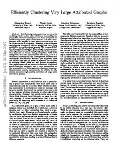
(FO) queries (i.e., non-recursive Datalog with negation) and an efficient method for explaining a (missing) answer using SQL. Our approach is based on the observation that typically only a part of provenance, which we call explanation in this work, is actually relevant for answering the user’s provenance question about the existence or absence of a result. Example 1. Consider the relation Train in Fig. 1 that stores train connections in the US. The Datalog rule r1 in Fig. 1 computes which cities can be reached with exactly one transfer, but not directly. We use the following abbreviations in provenance graphs: T = Train; n = New York; s = Seattle; w = Washington DC and c = Chicago. Given the result of this query, the user may be interested to know why he/she is able to reach Seattle from New York (W HY Q(n, s)) with one intermediate stop but not directly or why it is not possible to reach New York from Seattle in the same fashion (W HYNOT Q(s, n)). An explanation for either type of question should justify the existence (absence) of a result as the success (failure) to derive the result through the rules of the query. Furthermore, it should explain how the existence (absence) of tuples in the database caused the derivation to succeed (fail). Provenance graphs providing this type of justification for W HY Q(n, s) and W HYNOT Q(s, n) are shown in Fig. 2 and Fig. 3, respectively. There are three types of graph nodes: rule nodes (boxes labeled with a rule identifier and the constant arguments of a rule derivation), goal nodes (rounded boxes labeled with a rule identifier and the goal’s position in the rule’s body), and tuple

Q(s, n) r1 (s, n, w) g11 (s, w) T (s, w)

g12 (w, n) T (w, n)

r1 (s, n, c) g12 (c, n) T (c, n)

r1 (s, n, s) g11 (s, s)

r1 (s, n, n)

g12 (s, n)

T (s, s)

g11 (s, n)

T (s, n)

g12 (n, n) T (n, n)

Fig. 3: Provenance graph explaning W HYNOT Q(s, n)

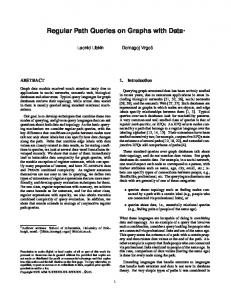
nodes (ovals). In these provenance graphs, nodes are either colored as green (successful/existing) or red (failed/missing). Example 2. Consider the explanation (provenance graph in Fig. 2) for question W HY Q(n, s). Seattle can be reached from New York by either stopping in Washington DC or Chicago and there is no direct connection between these two cities. These two options correspond to two successful derivations for rule r1 with X=n, Y =s, and Z=w (or Z=c, respectively). In the provenance graph, there are two rule nodes denoting these successful derivations of Q(n, s) by rule r1 . A derivation is successful if all goals in the body evaluate to true, i.e., a successful rule node is connected to successful goal nodes (e.g., r1 is connected to g11 , the 1st goal in the rule’s body). A positive (negated) goal is successful if the corresponding tuple is (is not) in the database. Thus, a successful goal node is connected to the node corresponding to the existing (green) or missing (red) tuple justifying the goal, respectively. Supporting negation and missing answers is quite challenging, because we need to enumerate all potential ways of deriving a missing answer (or intermediate result corresponding to a negated subgoal) and explain why each of these derivations has failed. An important question in this respect is how to bound the set of missing answers to be considered. Under the open world assumption, provenance would be infinite. Using the closed world assumption, only values that exist in the database or are postulated by the query are used to construct missing tuples. As is customary in Datalog, we refer to this set of values as the active domain adom(I) of a database instance I. We will revisit the assumption that all derivations with constants from adom(I) are meaningful later on. Example 3. The explanation for W HYNOT Q(s, n) is shown in Fig. 3, i.e., why it is not true that New York is reachable from Seattle with exactly one transfer, but not directly. The tuple Q(s, n) is missing from the query result because all potential ways of deriving this tuple through the rule r1 have failed. In this example, adom(I)={c, n, s, w} and, thus, there exist four failed derivations of Q(s, n) choosing either of these cities as the intermediate stop between Seattle and New York. A rule derivation fails if at least one goal in the body evaluates to false. In the provenance graph, only failed goals are connected to the failed rule derivations explaining missing answers. Failed positive goals in the body of a failed rule are explained by missing tuples (red tuple nodes). For instance, we cannot reach New York from Seattle with an intermediate stop in Washington DC (the first failed rule derivation from the left

in Fig. 3) because there exists no connection from Seattle to Washington DC (a tuple node T(s, w) in red), and Washington DC to New York (a tuple node T(w, n) in red). Note that the successful goal ¬ T(s, n) (there is no direct connection from Seattle to New York) does not contribute to the failure of this derivation and, thus, is not part of the explanation. A failed negated goal is explained by an existing tuple in the database. That is, if a tuple (s, n) would exist in the Train relation, then an additional failed goal node g13 (s, n) would be part of the explanation and be connected to each failed rule derivation. Overview and Contributions. Provenance games [20], a game-theoretical formalization of provenance for first-order (FO) queries, also supports queries with negation. However, the approach is computationally expensive, because it requires instantiation of a provenance graph explaining all answers and missing answers. For instance, the provenance graph produced by this approach for our toy example already contains more than 64 (=43 ) nodes (i.e., only counting nodes corresponding to rule derivations), because there are 43 ways of binding values from adom(I)={c, n, s, w} to the 3 variables (X, Y , and Z) of the rule r1 . Typically, most of the nodes will not end up being part of the explanation for the user’s provenance question. To efficiently compute the explanation, we introduce a new Datalog program which computes part of the provenance graph of an explanation bottom-up. Evaluating this program over instance I returns the edge relation of an explanation. The main driver of our approach is a rewriting of Datalog rules that captures successful and failed rule derivations. This rewriting replaces the rules of the program with so-called firing rules. Firing rules for positive queries were first introduced in [19]. These rules are similar to other query instrumentation techniques that have been used for provenance capture such as the rewrite rules of Perm [13]. One of our major contributions is to extend this concept for negation and failed rule derivations which is needed to support Datalog with negation and missing answers. Firing rules provide sufficient information for constructing explanations. However, to make this approach efficient, we need to avoid capturing rule derivations that will not contribute an explanation, i.e., they are not connected to the nodes corresponding to the provenance question in the provenance graph. We achieve this by propagating information from the user’s provenance question throughout the query to prune rule derivations early on 1) if they do not agree with the constants in the question or 2) if we can determine that based on their success/failure status they cannot be part of the explanation. For instance, in our running example, Q(n, s) can only be connected to successful derivations of the rule r1 with X=n and Y =s. We have presented a proof-of-concept version of our approach as a poster [21]. Our main contributions are: • We introduce a provenance graph model for full firstorder (FO) queries, expressed as non-recursive Datalog queries with negation (or Datalog for short). • We extend the concept of firing rules to support negation and missing answers. • We present an efficient method for computing explana-

tions to provenance questions. Unlike the solution in [20], our approach avoids unnecessary work by focusing the computation on relevant parts of the provenance graph. • We prove the correctness of our algorithm that computes the explanation to a provenance question. • We present a full implementation of our approach in the GProM [1] system. Using this system, we compile Datalog into relational algebra expressions, and translate the expressions into SQL code that can be executed by a standard relational database backend. The remainder of this paper is organized as follows. We formally define the problem in Sec. II, discuss related work in Sec. III, and present our approach for computing explanations in Sec. IV. We then discuss our implementation (Sec. V), present experiments (Sec. VI), and conclude in Sec. VII. II. P ROBLEM D EFINITION We now formally define the problem addressed in this work: how to find the subgraph of a provenance graph for a given query (input program) P and instance I that explains existence/absence of a tuple in/from the result of P . A. Datalog A Datalog program P consists of a finite set of rules ~ :− R1 (X ~1 ), . . . , Rn (X~n ) where X ~ j denotes a tuple ri : R(X) of variables and/or constants. We assume that the rules of ~ is the head of the a program are labeled r1 to rm . R(X) ~1 ), . . . , Rn (X~n ) is the body rule, denoted head(ri ), and R1 (X ~ j ) is a goal). We use vars(ri ) to denote the (each Rj (X set of variables in ri . In this paper, consider non-recursive ~ j ) in the body are literals, Datalog with negation, so goals Rj (X ~ ~ j ). Recursion is not i.e., atoms A(Xj ) or their negation ¬A(X allowed. All rules r of a program have to be safe, i.e., every variable in r must occur positively in r’s body (thus, head variables and variables in negated goals must also occur in a positive goal). For example, Fig. 1 shows a Datalog query with a single rule r1 . Here, head(r1 ) is Q(X, Y ) and vars(r1 ) is {X, Y, Z}. The rule is safe since the head variables and the variables in the negated goal also occur positively in the body (X and Y in both cases). The set of relations in the schema over which P is defined is referred to as the extensional database (EDB), while relations defined through rules in P form the intensional database (IDB), i.e., the IDB relations are those defined in the head of rules. We require that P has a distinguished IDB relation Q, called the answer relation. Given P and instance I, we use P (I) to denote the result of P evaluated over I. Note that P (I) includes the instance I, i.e., all EDB atoms that are true in I. For an EDB or IDB predicate R, we use R(I) to denote the instance of R computed by P and R(t) ∈ P (I) to denote that t ∈ R(I) according to P . We use adom(I) to denote the active domain of instance I, i.e., the set of all constants that occur in I. Similarly, we use adom(R.A) to denote the active domain of attribute A of relation R. In the following, we make use of the concept of a rule derivation. A derivation of a rule r is an assignment of variables in r to constants from adom(I). For a rule with n

variables, we use r(c1 , . . . , cn ) to denote the derivation that is the result of binding Xi =ci . We call a derivation successful wrt. an instance I if each atom in the body of the rule is true in I and failed otherwise. B. Negation and Domains To be able to explain why a tuple is missing, we have to enumerate all failed derivations of this tuple and, for each such derivation, explain why it failed. As mentioned in Sec. I, the question is what is a feasible set of potential answers to be considered as missing. While the size of why-not provenance is typically infinite under the open world assumption, we have to decide how to bound the set of missing answers in the closed world assumption. We propose a simple, yet general, solution by assuming that each attribute of an IDB or EDB relation has an associated domain. Definition 1 (Domain Assignment). Let S = {R1 , . . . , Rn } be a database schema where each Ri (A1 , . . . , Am ) is a relation schema. Given an instance I of S, a domain assignment dom is a function that associates with each attribute R.A a domain of values. We require dom(R.A) ⊇ adom(R.A). In our approach, the user specifies each dom(R.A) as a query dom R.A that returns the set of admissible values for the domain of attribute R.A. We provide reasonable defaults to avoid forcing the user to specify dom for every attribute, e.g., dom(R.A)=adom(R.A) for unspecified dom R.A . These associated domains fulfill two purposes: 1) to reduce the size of explanations and 2) to avoid semantically meaningless answers. For instance, if there would exist another attribute Price in the relation Train in Fig. 1, then adom(I) would also include all the values that appear in this attribute. Thus, some failed rule derivations for r1 would assign prices to the variable representing intermediate stops. Different attributes may represent the same type of entity (e.g., fromCity and toCity in our example) and, thus, it would make sense to use their combined domain values when constructing missing answers. For now, we leave it up to the user to specify attribute domains. Using techniques for discovering semantic relationships among attributes to automatically determine feasible attribute domains is an interesting avenue for future work. When defining provenance graphs in the following, we are only interested in rule derivations that use constants from the associated domains of attributes accessed by the rule. Given a rule r and variable X used in this rule, let attrs(r, X) denote the set of attributes that variable X is bound to in the body of the rule. For instance, in Fig. 1, attrs(r1 , Z)={Train.fromCity, Train.toCity}. We say a rule derivation r(c1 , . . . , cn ) is domain grounded iff ci ∈ T A∈attrs(r,Xi ) dom(A) for all i ∈ {1, . . . , n}. C. Provenance Graphs Provenance graphs justify the existence or absence of a query result based on the success or failure of derivations using a query’s rules, respectively. They also explain how the existence or absence of tuples in the database caused

derivations to succeed or fail, respectively. Here, we present a constructive definition of provenance graphs that provide this type of justification. Nodes in these graphs carry two types of labels: 1) a label that determines the node type (tuple, rule, or goal) and additional information, e.g., the arguments and rule identifier of a derivation; 2) the success/failure status of nodes. Definition 2 (Provenance Graph). Let P be a first-order (FO) query, I a database instance, dom a domain assignment for I, and L the domain containing all strings. The provenance graph PG(P, I) is a graph (V, E, L, S) with nodes V , edges E, and node labelling functions L : V → L and S : V → {T , F }. We require that ∀v, v 0 ∈ V : L(v) = L(v 0 ) → v = v 0 . PG(P, I) is defined as follows: • Tuple nodes: For each n-ary EDB or IDB predicate R and tuple (c1 , . . . , cn ) of constants from the associated domains (ci ∈ dom(R.Ai )), there exists a node v labeled R(c1 , . . . , cn ). S(v) = T iff R(c1 , . . . , cn ) ∈ P (I) and S(v) = F otherwise. • Rule nodes: For every successful domain grounded derivation ri (c1 , . . . , cn ), there exists a node v in V labeled ri (c1 , . . . , cn ) with S(v) = T . For every failed domain grounded derivation ri (c1 , . . . , cn ) where head(ri (c1 , . . . , cn )) 6∈ P (I), there exists a node v as above but with S(v) = F . In both cases, v is connected to the tuple node head(ri (c1 , . . . , cn )). • Goal nodes: Let v be the node corresponding to a derivation ri (c1 , . . . , cn ) with m goals. If S(v) = T , then for all j ∈ {1, . . . , m}, v is connected to a goal node vj labeled gij with S(vj ) = T . If S(v) = F , then for all j ∈ {1, . . . , m}, v is connected to a goal node vj with S(vj ) = F if the j th goal is failed in ri (c1 , . . . , cn ). Each goal is connected to the corresponding tuple node. Our provenance graphs model query evaluation by construction. A tuple node R(t) is successful in PG(P, I) iff R(t) ∈ P (I). This is guaranteed, because each tuple built from values of the associated domain exists as a node v in the graph and its label S(v) is decided based on R(t) ∈ P (I). Furthermore, there exists a successful rule node r(~c) ∈ PG(P, I) iff the derivation r(~c) succeeds for I. Likewise, a failed rule node r(~c) exists iff the derivation r(~c) is failed over I and head(r(~c)) 6∈ P (I). Fig. 2 and 3 show subgraphs of PG(P, I) for the query from Fig. 1. Since Q(n, s) ∈ P (I) (Fig. 2), this tuple node is connected to all successful derivations with Q(n, s) in the head which in turn are connected to goal nodes for each of the three goals of rule r1 . Q(s, n) ∈ / P (I) (Fig. 3) and, thus, its node is connected to all failed derivations with Q(s, n) as a head. Here, we have assumed that all cities can be considered as starting and end points of missing train connections, i.e., both dom(T.fromCity) and dom(T.toCity) are defined as adom(T.fromCity) ∪ adom(T.toCity). Thus, we have considered derivations r1 (s, n, Z) for Z ∈ {c, n, s, w}. An important characteristic of our provenance graphs is that each node v in a graph is uniquely identified by its label L(v). Thus, common subexpressions are shared leading to more

compact provenance graphs. For instance, observe that the node g13 (n, s) is shared by two rule nodes in the explanation shown in Fig 2. D. Questions and Explanations Recall that the problem we address in this work is how to explain the existence or absence of (sets of) tuples using provenance graphs. Such a set of tuples is called a provenance question (PQ) in this paper. The two questions presented in Example 1 use constants only, but we also support provenance questions with variables, e.g., for a question Q(n, X) we would return all explanations for existing or missing tuples where the first attribute is n, i.e., why or why-not a city X can be reached from New York with one transfer, but not directly. We say a tuple t0 of constants matches a tuple t of variables and constants written as t0 2 t if we can unify t0 with t, i.e., we can equate t0 with t by applying a valuation that substitutes variables in t with constants from t0 . Definition 3 (Provenance Question). Let P be a query, I an instance, and Q an IDB predicate. A provenance question PQ is an atom Q(t) where t = (v1 , . . . , vn ) is a tuple consisting of variables and constants from the associated domain (dom(Q.A) for each attribute Q.A). W HY Q(t) and W HYNOT Q(t) restrict the question to existing and missing tuples t0 2 t, respectively. In Example 1, we have presented subgraphs of PG(P, I) as explanations for PQs, implicitly claiming that these subgraphs are sufficient for explaining the PQ. Below, we formally define this type of explanation. Definition 4 (Explanation). The explanation E XPL(P, Q(t), I) for Q(t) (PQ) according to P and I, is the subgraph of PG(P, I) containing only nodes that are connected to at least one node Q(t0 ) where t0 2 t. For W HY Q(t), only existing tuples t0 are considered to match t. For W HYNOT Q(t) only missing tuples are considered to match t. Given this definition of explanation, note that 1) all nodes connected to a tuple node matching the PQ are relevant for computing this tuple and 2) only nodes connected to this node are relevant for the outcome. Consider t0 where t0 2 t for a Q(t) (PQ). If Q(t0 ) ∈ P (I), then all successful derivations with head Q(t0 ) justify the existence of t0 and these are precisely the rule nodes connected to Q(t0 ) in PG(P, I). If Q(t0 ) 6∈ P (I), then all derivations with head Q(t0 ) have failed and are connected to Q(t) in the provenance graph. Each such derivation is connected to all of its failed goals which are responsible for the failure. Now, if a rule body references IDB predicates, then the same argument can be applied to reason that all rules directly connected to these tuples explain why they (do not) exist. Thus, by induction, the explanation contains all relevant tuple and rule nodes that explain the PQ. III. R ELATED W ORK Our provenance graphs have strong connections to other provenance models for relational queries, most importantly

provenance games and the semiring framework, and to approaches for explaining missing answers. Provenance Games. Provenance games [20] model the evaluation of a given query (input program) P over an instance I as a 2-player game in a way that resembles SLD(NF) resolution. If the position (a node in the game graph) corresponding to a tuple t is won (the player starting in this position has a winning strategy), then t ∈ P (I) and if the position is lost, then t 6∈ P (I). By virtue of supporting negation, provenance games can uniformly answer why and why-not questions for queries with negation. However, provenance games may be hard to comprehend for non-power users as they require some background in game theory to be understood, e.g., the won/lost status of derivations in a provenance game is contrary to what may be intuitively expected. That is, a rule node is lost if the derivation is successful. The status of rule nodes in our provenance graphs matches the intuitive expectation (e.g., the rule node is successful if the derivation exists). K¨ohler et al. [20] also present an algorithm that computes the provenance game for P and I. However, this approach requires instantiation of the full game graph (which enumerates all existing and missing tuples) and evaluation of a recursive Datalog¬ program over this graph using the well-founded semantics [11]. In constrast, our approach computes explanations that are succinct subgraphs containing only relevant provenance. We use bottom-up evaluation instrumented with firing rules to capture provenance. Furthermore, we enable the user to restrict provenance for missing answers. Database Provenance. Several provenance models for database queries have been introduced in related work, e.g., see [7], [18]). The semiring annotation framework generalizes these models for positive relational algebra (and, thus, positive non-recursive Datalog). In this model, tuples in a relation are annotated with elements from a commutative semiring K. An essential property of the K-relational model is that semiring N[X], the semiring of provenance polynomials, generalizes all other semirings. It has been shown in [20] that provenance games generalize N[X] for positive queries and, thus, all other provenance models expressible as semirings. Since our graphs are equivalent to provenance games in the sense that there exist lossless transformations between both models (the discussion is beyond the scope of this paper), our graphs also encode N[X]. Provenance graphs which are similar to our graphs restricted to positive queries have been used as graph representations of semiring provenance (e.g., see [8], [9], [18]). Both our graphs and the boolean circuits representation of semiring provenance [9] explicitly share common subexpressions in the provenance. However, while these circuits support recursive queries, they do not support negation. Exploring the relationship of provenance graphs for queries with negation and m-semirings (semirings with support for set difference) is an interesting avenue for future work. Justifications for logic programs [23] are also closely related. Why-not and Missing Answers. Approaches for explaining missing answers can be classified based on whether they

explain a missing answer based on the query [3], [4], [6], [25] (i.e., which operators filter out tuples that would have contributed to the missing answer) or based on the input data [16], [17] (i.e., what tuples need to be inserted into the database to turn the missing answer into an answer). The missing answer problem was first stated for query-based explanations in the seminal paper by Chapman et al. [6]. Huang et al. [17] first introduced an instance-based approach. Since then, several techniques have been developed to exclude spurious explanations, to support larger classes of queries [16], and to support distributed Datalog systems in Y! [26]. The approaches for instance-based explanations (with the exception of Y!) have in common that they treat the missing answer problem as a view update problem: the missing answer is a tuple that should be inserted into a view corresponding to the query and this insert has to be translated to an insert into the database instance. An explanation is then one particular solution to this view update problem. In contrast to these previous works, our provenance graphs explain missing answers by enumerating all failed rule derivations that justify why the answer is not in the result. Thus, they are arguably a better fit for use cases such as debugging queries, where in addition to determining which missing inputs justify a missing answer, the user also needs to understand why derivations have failed. Furthermore, we do support queries with negation. Importantly, solutions for view update missing answer problems can be extracted from our provenance graphs. Thus, in a sense, provenance graphs with our approach generalize some of the previous approaches (for the class of queries supported, e.g., we do not support aggregation yet). Interestingly, recent work has shown that it may be possible to generate more concise summaries of provenance games [12], [24] which is particularly useful for negation and missing answers to deal with the potentially large size of the resulting provenance. Similarly, some missing answer approaches [16] use c-tables to compactly represent sets of missing answers. These approaches are complementary to our work. Computing Provenance Declaratively. The concept of rewriting a Datalog program using firing rules to capture provenance as variable bindings of rule derivations was introduced by K¨ohler et al. [19] for provenance-based debugging of positive Datalog queries. These rules are also similar to relational implementations of provenance polynomials in Perm [13], LogicBlox [14], and Orchestra [15]. Zhou et al. [27] leverage such rules for the distributed ExSPAN system using either full propagation or reference based provenance. An extension of firing rules for negation is the main enabler of our approach. IV. C OMPUTING E XPLANATIONS Recall from Sec. I that our approach generates a new Datalog program GP(P, Q(t), I) by rewriting a given query (input program) P to return the edge relation of explanation E XPL(P, Q(t), I) for a provenance question Q(t) (PQ). In this section, we explain how to generate the program GP(P, Q(t), I) using the following steps:

1. We unify the input program P with the PQ by propagating the constants in t top-down throughout the program to be able to later prune irrelevant rule derivations. 2. Afterwards, we determine for which nodes in the graph we can infer their success/failure status based on the PQ. We model this information as annotations on heads and goals of rules and propagate these annotations top-down. 3. Based on the annotated and unified version created in the previous steps, we generate firing rules that capture variable bindings for successful and failed rule derivations. 4. To be in the result of one of the firing rules obtained in the previous step is a necessary, but not sufficient, condition for the corresponding PG(P, I) fragment to be connected to a node matching the PQ. To guarantee that only relevant fragments are returned, we introduce additional rules that check connectivity to confirm whether each fragment is connected. 5. Finally, we create rules that generate the edge relation of the provenance graph (i.e., E XPL(P, Q(t), I)) based on the rule binding information that the firing rules have captured. In the following, we will explain each step in detail and illustrate its application based on the question W HY Q(n, s) from Example 1, i.e., why is New York connected to Seattle via a train connection with one intermediate stop, but is not directly connected to Seattle. A. Unify the Program with PQ The node Q(n, s) in the provenance graph (Fig. 2) is only connected to rule derivations which return Q(n, s). For instance, if variable X is bound to another city x (e.g., Chicago) in a derivation of the rule r1 , then this rule cannot return the tuple (n, s). This reasoning can be applied recursively to replace variables in rules with constants. That is, we unify the rules in the program top-down with the PQ. This step may produce multiple duplicates of a rule with different bindings. We use superscripts to make explicit the variable binding used by a replica of a rule. Example 4. Given the question W HY Q(n, s), we unify the single rule r1 using the assignment (X=n, Y =s): (X=n,Y =s)

r1

: Q(n, s) :− T(n, Z), T(Z, s), ¬ T(n, s)

We may have to create multiple partially unified versions of a rule or an EDB atom. For example, to explore successful derivations of Q(n, s) we are interested in both train connections from New York to some city (T(n, Z)) and from any city to Seattle (T(Z, s)). Furthermore, we need to know whether there is a direct connection from New York to Seattle (T(n, s)). The general idea of this step is motivated by [2] which introduced “magic sets”, an approach for rewriting logical rules to cut down irrelevant facts by using additional predicates called “magic predicates”. Similar techniques exist in standard relational optimization under the name of predicate move around. We use the technique of propagating variable bindings in the query to restrict the computation based on the user’s interest. This approach is correct because if we bind a variable in the head of rule, then only rule derivations

Algorithm 1 Unify Program With PQ 1: procedure U NIFY P ROGRAM(P , Q(t)) 2: todo ← [Q(t)] 3: done ← {} 4: PU = [] 5: while todo 6= [] do 6: a ← POP(todo) 7: INSERT (done, a) 8: rules ← GET RULES F OR ATOM(P, a) 9: for all r ∈ rules do 10: unRule ← UNIFY RULE(r, a) 11: PU ← PU :: unRule 12: for all g ∈ body(unRule) do 13: if g 6∈ done then todo ← todo :: g 14: return PU

that agree with this binding can derive tuples that agree with this binding. Based on this unification step, we know which bindings may produce fragments of PG(P, I) that are relevant for explaining the PQ. The algorithm implementing this step is given as Algorithm 1. B. Add Annotations based on Success/Failure For W HY and W HYNOT questions, we only consider tuples that are existing and missing, respectively. Based on this information, we can infer restrictions on the success/failure status of nodes in the provenance graph that are connected to PQ node(s) (belong to the explanation). We store these restrictions as annotations T , F , and F /T on heads and goals of rules. Here, T indicates that we are only interested in successful nodes, F that we are only interested in failed nodes, and F /T that we are interested in both. These annotations are determined using a top-down propagation seeded with the PQ. Example 5. Continuing with our running example question W HY Q(n, s), we know that Q(n, s) is successful because the tuple is in the result (Fig. 1). This implies that only successful rule nodes and their successful goal nodes can be connected to this tuple node. Note that this annotation does not imply that the rule r1 would be successful for every Z (i.e., every intermediate stop between New York and Seattle). It only indicates that it is sufficient to focus on successful rule derivations since failed ones cannot be connected to Q(n, s). (X=n,Y =s),T

r1

: Q(n, s)T :− T(n, Z)T , T(Z, s)T , ¬ T(n, s)T

We now propagate the annotations of the goals in r1 throughout the program. That is, for any goal that is an IDB predicate, we propagate its annotation to the head of all rules deriving the goal’s predicate and, then, propagate these annotations to the corresponding rule bodies. Note that the inverted annotation is propagated for negated goals. For instance, if T would be an IDB predicate, then the annotation on the goal ¬ T(n, s)T would be propagated as follows. We would annotate the head of all rules deriving T(n, s) with F , because Q(n, s) can only exist if T(n, s) does not exist. Partially unified atoms (such as T(n, Z)) may occur in both negative and positive goals of the rules of the program.

Algorithm 2 Success/Failure Annotations 1: procedure A NNOT P ROGRAM(PU , Q(t)) 2: state ← typeof (Q(t)) 3: todo ← [Q(t)state ] 4: done ← {} 5: PA = [] 6: while todo 6= [] do 7: a ← POP(todo) 8: state ← typeof (a) 9: INSERT(done, a) 10: rules ← GET U N RULES F OR ATOM(P, a) 11: for all r ∈ rules do 12: annotRule ← ANNOT RULE(r, state) 13: PA ← PA :: annotRule 14: for all g ∈ body(annotRule) do 15: if state = F then 16: newstate ← F /T 17: else 18: newstate ← state 19: if IS N EGATED(g) then 20: newstate ← SWITCH S TATE(state) 21: 22: 23: 24: 25: 26:

if g newstate 6∈ done ∧ IS IDB(g) then todo ← todo :: g newstate for all r ∈ PA do if typeof (r) = F /T then PA ← REMOVE A NNOTATED RULES(PA , r, {F , T }) return PA

We denote such atoms using a F /T annotation. The use of these annotations will become more clear in the next subsection when we introduce firing rules. The pseudocode for the algorithm that determines these annotations is given as Algorithm 2. In short: 1) Annotate the head of all rules deriving tuples matching the question with T (why) or F (why-not). 2) Repeat the following steps until a fixpoint is reached: a) Propagate the annotation of a rule head to goals in the rule body as follows: propagate T for T annotated heads and F /T for F annotated heads. b) For each annotated goal in the rule body, propagate its annotation to all rules that have this atom in the head. For negated goals, unless the annotation is F /T , we propagate the inverted annotation (e.g., F for T ) to the head of rules deriving the goal’s predicate. C. Creating Firing Rules To be able to compute the relevant subgraph of PG(P, I) (the explanation) for the provenance question PQ, we need to determine successful and/or failed rule derivations. Each rule derivation paired with the information whether it is successful over the given database instance (and which goals are failed in case it is not successful) corresponds to a certain subgraph. Successful rule derivations are always part of PG(P, I) for a given query (input program) P whereas failed rule derivations only appear if the tuple in the head failed, i.e., there are no successful derivations of any rule with this head. To capture the variable bindings of successful/failed rule derivations, we create “firing rules”. For successful rule derivations, a

FQ,T (n, s) :− Fr1 ,T (n, s, Z) Fr1 ,T (n, s, Z) :− FT,T (n, Z), FT,T (Z, s), FT,F (n, s) FT,T (n, Z) :− T(n, Z) FT,T (Z, s) :− T(Z, s) FT,F (n, s) :− ¬ T(n, s) Fig. 4: Example firing rules for W HY Q(n, s)

firing rule consists of the body of the rule (but using the firing version of each predicate in the body) and a new head predicate that contains all variables used in the rule. In this way, the firing rule captures all the variable bindings of a rule derivation. Furthermore, for each IDB predicate R that occurs as a head of a rule r, we create a firing rule that has the firing version of predicate R in the head and a firing version of the rules r deriving the predicate in the body. For EDB predicates, we create firing rules that have the firing version of the predicate in the head and the EDB predicate in the body. Example 6. Consider the annotated program in Example 5 for the question W HY Q(n, s). We generate the firing rules shown (X=n,Y =s),T in Fig. 4. The firing rule for r1 (the second rule from the top) is derived from the rule r1 by adding Z (the only existential variable) to the head, renaming the head predicate as Fr1 ,T , and replacing each goal with its firing version (e.g., FT,T for the two positive goals and FT,F for the negated goal). Note that negated goals are replaced with firing rules that have inverted annotations (e.g., the goal ¬ T(n, s)T is replaced with FT,F (n, s)). Furthermore, we introduce firing rules for EDB tuples (the three rules from the bottom in Fig. 4) As mentioned in Sec. III, firing rules for successful rule derivations have been used for declarative debugging of positive Datalog programs [19] and, for non-recursive queries, are essentially equivalent to rewrite rules that instrument a query to compute provenance polynomials [1], [13]. We extend firing rules to support queries with negation and capture missing answers. To construct a PG(P, I) fragment corresponding to a missing tuple, we need to find failed rule derivations with the tuple in the head and ensure that no successful derivations exist with this head (otherwise, we may capture irrelevant failed derivations of existing tuples). In addition, we need to determine which goals are failed for each failed rule derivation because only failed goals are connected to the node representing the failed rule derivation in the provenance graph. To capture this information, we add additional boolean variables - Vi for goal g i - to the head of a firing rule that record for each goal whether it failed or not. The body of a firing rule for failed rule derivations is created by replacing every goal in the body with its F /T firing version, and adding the firing version of the negated head to the body (to ensure that only bindings for missing tuples are captured). Firing rules capturing failed derivations use the F /T firing versions of their goals because not all goals of a failed derivation have

FQ,F (s, n) :− ¬ FQ,T (s, n)

Algorithm 3 Create Firing Rules

FQ,T (s, n) :− Fr1 ,T (s, n, Z)

1: procedure C REATE F IRING RULES(PA , Q(t)) 2: PF ire ← [] 3: state ← typeof (Q(t)) 4: todo ← [Q(t)state ] 5: done ← {} 6: while todo = 6 [] do . create rules for a predicate 7: R(t)σ ← POP(todo) σ 8: INSERT (done, R(t) ) 9: if IS EDB(R) then 10: C REATE EDBF IRING RULE(PF ire , R(t)σ ) 11: else 12: C REATE IDBN EG RULE(PF ire , R(t)σ ) 13: rules ← GET RULES(R(t)σ ) 14: for all r ∈ rules do . create firing rule for r 15: args ← (vars(r) − vars(head(r))) 16: args ← args(head(r)) :: args 17: C REATE IDBP OS RULE(PF ire , R(t)σ , r, args) 18: C REATE IDBF IRING RULE(PF ire , R(t)σ , r, args)

Fr1 ,F (s, n, Z, V1 , V2 , ¬ V3 ) :− FQ,F (s, n), FT,F/T (s, Z, V1 ), FT,F/T (Z, n, V2 ), FT,F/T (s, n, V3 ) Fr1 ,T (s, n, Z) :− FT,T (s, Z), FT,T (Z, n), FT,F (s, n) FT,F/T (s, Z, true) :− FT,T (s, Z) FT,F/T (s, Z, f alse) :− FT,F (s, Z) FT,T (s, Z) :− T(s, Z) FT,F (s, Z) :− dom T.toCity (Z), ¬ T(s, Z) Fig. 5: Example firing rules for W HYNOT Q(s, n)

to be failed and the failure status determines whether the corresponding goal node is part of the explanation. A firing rule capturing missing IDB or EDB tuples may not be safe, i.e., it may contain variables that only occur in negated goals. In fact, these variables should be restricted to the associated domains for the attributes the variables are bound to. Since the associated domain dom for an attribute R.A is given as an unary query dom R.A , we can use these queries directly in firing rules to restrict the values the variable is bound to. This is how we ensure that only missing answers formed from the associated domains are considered and that firing rules are always safe. Example 7. Reconsider the question W HYNOT Q(s, n) from Example 1. The firing rules generated for this question are shown in Fig. 5. We exclude the rules for the second goal T(Z, n) and the negated goal ¬ T(s, n) which are analogous to the rules for the first goal T(s, Z). Since Q(s, n) is failed (because tuple (s, n), i.e., New York cannot be reachable from Seattle with exactly one transfer, is not in the result), we are only interested in failed rule derivations of the rule r1 with X=s and Y =n. Furthermore, each rule node in the provenance graph corresponding to such a rule derivation will only be connected to failed subgoals. Thus, we need to capture which goals are successful or failed for each such failed derivation. This can be modelled through boolean variables V1 , V2 , and V3 (since there are three goals in the body) that are true if the corresponding goal is successful and false otherwise. The firing version Fr1 ,F (s, n, Z, V1 , V2 , ¬ V3 ) of r1 will contain all variable bindings for derivations of r1 such that Q(s, n) is the head (i.e., guaranteed by adding FQ,F (s, n) to the body), the rule derivations are failed, and the ith goal is successful or failed for this binding iff Vi is true or false, respectively. To produce all these bindings, we need rules capturing successful and failed tuple nodes for each subgoal of the rule r1 . We denote such rules using a F /T annotation and use a boolean variable (true or false) to record whether a tuple exists (e.g., FT,F/T (s, Z, true) :− FT,T (s, Z) is one of these rules). Negated goals are dealt with by negating this boolean variable, i.e., the goal is successful if the corresponding tuple does not exist. For instance, FT,F/T (s, n, f alse) represents the fact that

19:

return PF ire

tuple T(s, n) (a direct train connection from Seattle to New York) is missing. This causes the third goal of r1 to succeed for any derivation where X=s and Y =n. For each partially unified EDB atom annotated with F /T , we create four rules: one for existing tuples (e.g., FT,T (s, Z) :− T(s, Z)), one for the failure case (e.g., FT,F (s, Z) :− dom T.toCity (Z), ¬ T(s, Z)), and two for the F /T firing version. For the failure case, we use predicate dom T.toCity to only consider missing tuples (s, Z) where Z is a value from the associated domain of this attribute. The algorithm that creates the firing rules for an annotated input query is shown as Algorithm 3 (the pseudocode for the subprocedures is given as Algorithm 4). It maintains a list of annotated atoms that need to be processed which is initialized with the Q(t) (PQ). For each such atom R(t)σ (here σ is the annotation of the atom), it creates firing rules for each rule r that has this atom as a head and a positive firing rule for R(t). Furthermore, if the atom is annotated with F /T or F , then additional firing rules are added to capture missing tuples and failed rule derivations. EDB atoms. For an EDB atom R(t)T , we use procedure CREATE EDBF IRING RULE to create one rule FR,T (t) :− R(t) that returns tuples from relation R that matches t. For missing tuples (R(t)F ), we extract all variables from t (some arguments may be constants propagated during unification) and create a rule that returns all tuples that can be formed from values of the associated domains of the attributes these variables are bound to and do not exist in R. This is achieved by adding goals dom(Xi ) as explained in Example 7. ~1 ), . . . , gn (X~n ). If the Rules. Consider a rule r : R(t) :− g1 (X head of r is annotated with T , then we create a rule with ~ where X ~ = vars(r) and the same body as r head Fr,T (X) except that each goal is replaced with its firing version with appropriate annotation (e.g., T for positive goals). For rules annotated with F or F /T , we create one additional rule with ~ V ~ ) where X ~ is defined as above, and V ~ contains head Fr,F (X, Vi if the ith goal of r is positive and ¬ Vi otherwise. The body

Algorithm 4 Create Firing Rules Subprocedures σ

1: procedure C REATE EDBF IRING RULE(PF ire , R(t) ) 2: [X1 , . . . , Xn ] ← vars(t) 3: rT ← FR,T (t) :− R(t) 4: rF ← FR,F (t) :− dom(X1 ), . . . , dom(Xn ), ¬ R(t) 5: rF /T −1 ← FR,F/T (t, true) :− FR,T (t) 6: rF /T −2 ← FR,F/T (t, f alse) :− FR,F (t) 7: if σ = T then 8: PF ire ← PF ire :: rT 9: else if σ = F then 10: PF ire ← PF ire :: rT :: rF 11: else 12: PF ire ← PF ire :: rT :: rF :: rF /T −1 :: rF /T −2 1: procedure C REATE IDBN EG RULE(PF ire , R(t)σ ) 2: [X1 , . . . , Xn ] ← vars(t) 3: if σ 6= T then 4: rnew ← FR,F (t) :− dom(X1 ), . . . , dom(Xn ), ¬ FR,T (t) 5: PF ire ← PF ire :: rnew 6: if σ = F /T then 7: rT ← FR,F/T (t, true) :− FR,T (t) 8: rF ← FR,F/T (t, f alse) :− FR,F (t) 9: PF ire ← PF ire :: rT :: rF 1: procedure C REATE IDBP OS RULE(PF ire , R(t)σ , r, args) 2: rpred ← FR,T (t) :− Fr,T (args) 3: PF ire ← PF ire :: rpred 1: procedure C REATE IDBF IRING RULE(PF ire , R(t)σ , r, args) 2: bodynew ← [] ~ ∈ body(r) do 3: for all gi (X) 4: σgoal ← T 5: if IS N EGATED(g) then 6: σgoal ← F 7: 8: 9: 10: 11: 12: 13: 14: 15: 16: 17: 18: 19: 20: 21: 22: 23: 24: 25: 26:

~ gnew ← Fpred(gi ),σgoal (X) bodynew ← bodynew :: gnew ~ T 6∈ (done ∪ todo) ∧ σ = T then if g(X) ~ σgoal todo ← todo :: g(X) rnew ← Fr,T (args) :− bodynew PF ire ← PF ire :: rnew if σ 6= T then for all gi ∈ body(r) do if IS N EGATED(gi ) then args ← args :: ¬bi else args ← args :: bi bodynew ← [] ~ ∈ body(r) do for all gi (X) ~ bi ) gnew ← Fpred(gi ),F/T (X, bodynew ← bodynew :: gnew ~ F /T 6∈ (done ∪ todo) then if g(X) ~ σgoal todo ← todo :: g(X) rnew ← Fr,σ (args) :− bodynew PF ire ← PF ire :: rnew

of this rule contains the F /T version of every goal in r’s body plus an additional goal FR,F to ensure that the head atom is failed. As an example for this type of rule, consider the third rule from the top in Fig. 5. IDB atoms. For each rule r with head R(t), we create a rule ~ where X ~ is the concatenation of t with all FR,T (t) :− Fr,T (X) existential variables from the body of r. IDB atoms with F or F /T annotations are handled in the same way as EDB atoms

with these annotations. For each R(t)F , we create a rule with ¬ FR,T (t) in the body using the associated domain queries to restrict variable bindings. For R(t)F /T , we add two additional rules as shown in Fig. 5 for EDB atoms. Theorem 1 (Correctness of Firing Rules). Let P be an input program, r denote a rule of P with m goals, and PF ire be the firing version of P . We use r(t) |= P (I) to denote that the rule derivation r(t) is successful in the evaluation of program P over I. The firing rules for P correctly determine existence of tuples, successful rule derivations, and failed rule derivations for missing answers: • • • •

FR,T (t) ∈ PF ire (I) ↔ R(t) ∈ P (I) FR,F (t) ∈ PF ire (I) ↔ R(t) 6∈ P (I) Fr,T (t) ∈ PF ire (I) ↔ r(t) |= P (I) ~ ) ∈ PF ire (I) ↔ r(t) 6|= P (I) ∧ head(r(t)) 6∈ Fr,F (t, V P (I) and for i ∈ {1, . . . , m} we have that Vi is false iff ith goal fails in r(t).

Proof: We prove Theorem 1 by induction over the structure of a program. For the base case, we consider programs of “depth” 1, i.e., only EDB predicates are used in rule bodies. Then, we prove correctness for programs of depth n + 1 based on the correctness of programs of depth n. We define the depth d of predicates, rules, and programs as follows: 1) for all EDB predicates R, we define d(R) = 0; 2) for an IDB predicate R, we define d(R) = maxhead(r)=R d(r), i.e., the maximal depth among all rules r with head(r) = R; 3) the depth of a rule r is d(r) = maxR∈body(r) d(R) + 1, i.e., the maximal depth of all predicates in its body plus one; 4) the depth of a program P is the maximum depth of its rules: d(P ) = maxr∈P d(r). 1) Base Case. Assume that we have a program P with depth ~ :− R(X ~1 ), . . . , R(X~n ). We first prove that the 1, e.g., r : Q(X) positive and negative versions of firing rules for EDB atoms are correct, because only these rules are used for the rules of depth 1 programs. A positive version of EDB firing rule FR,T creates a copy of the input relation R and, thus, a tuple t ∈ R iff t ∈ FR,T . For the negative version FR,F , all variables are bound to associated domains dom and it is explicitly checked that ~ is true. Finally, FR,F/T uses FR,T and FR,F to determine ¬ R(X) whether the tuple exists in R. Since these rules are correct, it follows that FR,F/T is correct. The positive firing rule for the rule r (Fr,T ) is correct since its body only contains positive and negative EDB firing rules (FR,T respective FR,F ) which are already known to be correct. The correctness of the positive firing version of a rule’s head predicate (FQ,T ) follows naturally from the correctness of Fr,T . The negative version of the rule ~ V ~ ) contains an additional goal (i.e., ¬ Q(X)) ~ and uses Fr,F (X, the firing version FR,F/T to return only bindings for failed derivations. Since FR,F/T has been proven to be correct, we only need to prove that the negative firing version of the head predicate of r is correct. For a head predicate with annotation F , we create two firing rules (FQ,T and FQ,F ). The rule FQ,T was already proven to be correct. FQ,F is also correct, because it contains only FQ,T and domain queries in the body which were already proven to be correct.

FQ,T (n, s) :− Fr1 ,T (n, s, Z) Fr1 ,T (n, s, Z) :− FT,T (n, Z), FT,T (Z, s), FT,F (n, s) FCr2 ,r11 ,T (n, Z) :− T(n, Z), Fr1 ,T (n, s, Z) FCr2 ,r21 ,T (Z, s) :− T(Z, s), Fr1 ,T (n, s, Z) FT,F (n, s) :− ¬ T(n, s) Fig. 6: Example firing rules with connectivity checks

2) Inductive Step. It remains to be shown that firing rules for programs of depth n + 1 are correct. Assume that firing rules for programs of depth up to n are correct. Let r be a firing rule of depth n + 1 in a program of depth n + 1. It follows that maxR∈body(r) d(R) ≤ n, otherwise r would be of a depth larger than n + 1. Based on the induction hypothesis, it is guaranteed that the firing rules for all these predicates are correct. Using the same argument as in the base case, it follows that the firing rule for r is correct.

Algorithm 5 Add Connectivity Joins 1: procedure A DD C ONNECTIVITY RULES(PF ire , Q(t)) 2: PF C ← [] 3: paths ← PATH S TARTING I N(PF ire , Q(t)) 4: for all p ∈ paths do 5: p ← FILTER RULE N ODES(p) ~1 )σ1 , rj (X ~2 )σ2 ) ∈ p do 6: for all e = (ri (X 7: goals ← GET M ATCHING G OALS(e) 8: for all gk ∈ goals do 9: gnew ← UNIFY H EAD(Fri ,σ1 (t1 ), gk , Frj ,σ2 (t2 )) 10: rnew ← FCrj ,rki ,σ2 (t2 ) :− body(Frj ,σ2 (t2 )), gnew 11: PF C ← PF C :: rnew 12: return PF C

Q(n, s)

T edge(fQ (n, s), frT1 (n, s, Z)) :− Fr1 ,T (n, s, Z)

edge(frT1 (n, s, Z), fgT1 (n, Z)) :− Fr1 ,T (n, s, Z)

r1 (n, s, Z)

1

g11 (n, Z) T (n, Z)

g12 (Z, s) T (Z, s)

g13 (n, s) T (n, s)

edge(fgT1 (n, Z), fTT (n, Z)) :− Fr1 ,T (n, s, Z) 1

edge(fgT3 (n, s), fTF (n, s)) :− Fr1 ,T (n, s, Z) 1

D. Connectivity Joins

Fig. 7: Example structure/rules for edge relation of explanation

To be in the result of firing rules is a necessary, but not sufficient, condition for the corresponding rule node to be connected to a PQ node in the explanation. Thus, to guarantee that only nodes connected to the PQ node(s) are returned, we have to check whether they are actually connected.

body of rj . Effectively, these rules check one hop at a time whether rule nodes in the provenance graph are connected to the nodes matching the PQ.

Example 8. Consider the firing rules for W HY Q(n, s) shown in Fig. 4. The corresponding rules with connectivity checks are shown in Fig. 6. All the rule nodes corresponding to Fr1 ,T (n, s, Z) are guaranteed to be connected to the PQ node Q(n, s). For sake of the example, assume that instead of using T, rule r1 uses an IDB relation R which is computed using another rule r2 : R(X, Y ) :− T(X, Y ). Consider the firing rule Fr2 ,T (n, Z) :− T(n, Z) created based on the second goal of r1 . Some provenance graph fragments computed by this rule may not be connected to Q(n, s). A tuple node R(n, c) for a constant c is only connected to the node Q(n, s) iff it is part of a successful binding of r1 . That is, for the node R(n, c) to be connected, there has to exist another tuple (c, s) in R. We check connectivity to Q(n, s) one hop at a time. This is achieved by adding the head of the firing rule for r1 to the body of the firing rule for r2 as shown in Fig. 6 (the second ~ to denote and third rule from the bottom). We use FCr2 ,rk1 ,T (X) th the firing rule for r2 connected to the k goal of rule r1 . Note that, this connectivity check is unnecessary for rules with only constants (the last rule in Fig. 6). Algorithm 5 traverses the query’s rules starting from the PQ to find all combinations of rules ri and rj such that the head of rj can be unified with a goal in the body of ri . We use the subprocedure FILTER RULE N ODES to prune rules containing only constants. For each such pair (ri , rj ) where the head of rj corresponds to the k th goal in the body of ri , we create ~ as follows. We unify the variables of the a rule FCrj ,rki ,T (X) k th goal in the firing rule for ri with the head variables of the firing rule for rj . All remaining variables of ri are renamed to avoid name clashes. We then add the unified head of ri to the

E. Computing the Edge Relation The program created so far captures all the information needed to generate the edge relation of the graph for the PQ. To compute the edge relation, we use Skolem functions to create node identifiers. The identifier of a node captures the type of the node (tuple, rule, or goal), assignments from variables to constants, and the success/failure status of the node, e.g., a tuple node T(n, s) that is successful would be represented as fTT (n, s). Each rule firing corresponds to a fragment of PG(P, I). For example, one such fragment is shown in Fig. 7 (left). Such a substructure is created through a set of rules: • • •

One rule creating edges between tuple nodes for the head predicate and rule nodes One rule for each goal connecting a rule node to that goal node (for failed rules only the failed goals are connected) One rule creating edges between each goal node and the corresponding EDB tuple node

The pseudocode for creating rules that return the edge relation is provided as Algorithm 6. Example 9. Consider the firing rules with connectivity joins from Example 8. Some of the rules for creating the edge relation for the explanation sought by the user are shown in Fig. 7 (on the right side). For example, each edge connecting the tuple node Q(n, s) to a successful rule node r1 (n, s, Z) is created by the top-most rule, the second rule creates an edge between r1 (n, s, Z) and g11 (n, Z), and so on.

Algorithm 6 Create Edge Relation 1: procedure C REATE E DGE R ELATION(PF C , Q(t)) 2: PM ← [] 3: todo ← [Q(t)] 4: done ← {} 5: while todo 6= [] do 6: R(t)σ ← POP(todo) 7: if R(t)σ ∈ done then 8: continue 9: done ← INSERT(done, R(t)σ ) 10: rules ← GET RULES(R(t)σ ) 11: for all r ∈ rules do 12: if IS EDB(R) then 13: if σ = T then 14: if IS N EGATED(g) then F 0 15: rg→R ← edge(fgT (t0 ), fR (t )) :− Fr,T (args) 16: else T 0 17: rg→R ← edge(fgT (t0 ), fR (t )) :− Fr,T (args)

Q(X) :- R(X,Y). WHY(Q(1)). Datalog Parser + Analyzer

Provenance Game Rewriter

Optimizer

SQL Code Generator

SQL Code Generator

SELECT * FROM ...

SELECT * FROM ...

Oracle

Postgres

Q(X) :- Fire(X,Y,Z). Fire(X,Y,Z) :- …

GProM

Datalog to Relational Algebra Translator SQL Code SQL Code Generator SQL Code Generator Generator

—————

Backend Backend Backend

Fig. 8: Implementation in GProM

contains nodes with arguments from the associated domain. Any edge returned by GP(P, Q(t), I) is strictly based on the structure of the input program and connects nodes that agree on variable bindings. Thus, each edge produced by 18: else GP(P, Q(t), I) will be contained in PG(P, I). 19: argsb ← b1 , . . . , bi−1 , f alse, bi+1 , . . . , bn 2. We now prove that the program GP(P, Q(t), I) returns 20: if IS N EGATED(g) then T 0 the set of edges of E XPL(P, Q(t), I). Assume that 21: rg→R ← edge(fgF (t0 ), fR (t )) :− Fr,F (args, argsbprecisely ) 22: else the Q(t) (PQ) only uses constants (the extension to PQ which F 0 (t )) :− Fr,F (args, argsbcontains ) 23: rg→R ← edge(fgF (t0 ), fR variables is immediate). Consider a rule of an input 24: PM ← PM :: rg→R program of depth 1 (i.e., only EDB predicates in the body 25: else of rules). For such a rule node to be connected to the node 26: σr = SWITCH S TATE(σ) Q(t), its head variables have to be bound to t (guaranteed by σ σr 27: rnew ← edge(fpred(r) (t), fr (t, . . .)) :− Fr,σ (t, . . .) the unification step in Sec. IV-A). Since the firing rules are 28: PM ← PM :: rnew known to be correct, this guarantees that exactly the rule nodes 29: for all g(t0 ) ∈ body(r) do 30: if IS N EGATED(g) then connected to the PQ node are generated. The propagation 31: σ 0 ← SWITCH S TATE(σ) of this unification to the firing rules for EDB predicates is 32: else correct, because only EDB nodes agreeing with this binding 0 33: σ ←σ 0 can be connected to such a rule node. However, propagating 34: todo ← todo :: g(t0 )σ constants is not sufficient since the firing rule for an EDB 35: if σ = T then 36: rr→g ← edge(frT (args), fgT (t0 )) :− Fr,T (args) predicate (e.g., R) may return irrelevant tuples, i.e., tuples that 37: else are not part of any rule derivations for Q(t) (e.g., there may 38: argsb ← b1 , . . . , bi−1 , f alse, bi+1 , . . . , bn not exist EDB tuples for other goals in the rule which share F F 0 39: rr→g ← edge(fr (args), fg (t )) :− Fr,F (args, argsb ) variables with the particular goal using predicate R). This is 40: PM ← PM :: rr→g checked by the connectivity joins (Sec. IV-D). If a tuple is 41: return PM returned by a connected firing rule, then the corresponding node is guaranteed to be connected to at least one rule node F. Correctness deriving PQ. Note that this argument does not rely on the fact We now state correctness of our approach for computing an that predicates in the body of a rule are EDB predicates. Thus, we can apply this argument in a proof by induction to show explanation E XPL(P, Q(t), I) for a provenance question. that, given that rules of depth up to n only produce connected Theorem 2 (Correctness). The result of a Datalog program rule derivations, the same holds for rules of depth n + 1. GP(P, Q(t), I) that rewrites a query (input program) P over instance I is the edge relation of E XPL(P, Q(t), I). V. I MPLEMENTATION Proof: For Theorem 2, we prove that 1) only edges from PG(P, I) are returned by the program GP(P, Q(t), I) and 2) the program returns precisely the set of edges of explanation E XPL(P, Q(t), I). 1. The constant values used as variable binding by the rules creating edges in GP(P, Q(t), I) are either constants that occur in the PQ or the result of rules which are evaluated over the instance I. Since only the rules for creating the edge relation create new values (through Skolem functions), it follows that any constant used in constructing a node argument exists in the associated domain. Recall that the PG(P, I) only

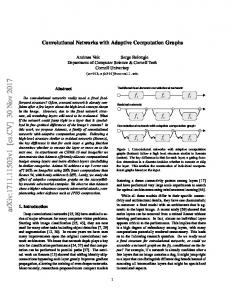
We have implemented the approach presented in Sec. IV in our provenance middleware called GProM [1] that executes provenance requests using a relational database backend (shown in Fig. 8). The system was originally developed to support provenance requests for SQL. We have extended the system to support Datalog enriched with syntax for stating provenance questions. The user provides a why or why-not question and the corresponding Datalog query as input. Our system parses and semantically analyzes this input. Schema information is gathered by querying the catalog of the backend database (e.g., to determine whether an EDB predicate with the

δ

πX,Y

./((X=X)∧(Y =Y ))

−

πX,Y

./(Z=Z)

πI→X,O→Z

Train

πI→Z,O→Y

Train Train

Fig. 9: Translation for rule r1

r1 : only2hop(X, Y ) :− DBLP(X, Z), DBLP(Z, Y ), ¬ DBLP(X, Y ) r2 : XwithYnotZ(X, Y ) :− DBLP(X, Y ), ¬ Q1 (X) r20 : Q1 (X) :− DBLP(X, ‘Svein Johannessen’) r3 : only3hop(X, Y ) :− DBLP(X, A), DBLP(A, B), DBLP(B, Y ), ¬ E1 (X), ¬ E2 (X) r30 : E1 (X) :− DBLP(X, Y )

expected arity exists). Modules for accessing schema information are already part of the GProM system, but a new semantic analysis component had to be developed to support Datalog. The algorithms presented in Sec. IV are applied to create the program GP(P, Q(t), I) which computes E XPL(P, Q(t), I). This program is translated into a relational algebra (RA) graph (GProM uses algebra graphs instead of trees to allow for sharing of common subexpressions). The algebra graph is then translated into SQL and sent to the backend database to compute the edge relation of the explanation for the PQ. Based on this edge relation, we then render a provenance graph (e.g., the graphs shown in Example 1 are actual results produced by the system).1 While it would certainly be possible to directly translate the Datalog program into SQL without the intermediate translation into RA, we choose to introduce this step to be able to leverage the existing heuristic and costbased optimizations for RA graphs built into GProM and use its library of RA to SQL translators. Our translation of first-order (FO) queries (a program with a distinguished answer relation) to RA is mostly standard. We first translate each rule into an algebra expression independently. Afterwards, we create expressions for IDB predicates as a union of the expressions for all rules with the predicates in the head. Finally, the algebra expressions for individual IDB predicates are connected into a single graph by replacing references to IDB predicates with their algebraic translation. Example 10. Consider the translation of the rule r1 from Fig. 1. The RA graph for r1 is shown in Fig. 9. The translations of the first two goals are joined to compute the variable bindings for the positive part of the query. The negated goal is translated into a set difference between the positive part projected on X, Y and relation Train. The remaining three operators (from the left) join the positive with the negative part, project on the head variables, and remove duplicates. VI. E XPERIMENTS We evaluate the performance of our solution over a coauthor graph relation extracted from DBLP (http://www.dblp. org/) as well as over the TPC-H decision support benchmark (http://www.tpc.org/tpch/default.asp). We compare our approach for computing explanations with the approach introduced for provenance games [20]. We call the provenance game approach Direct Method(DM), because it directly constructs the full provenance graph. We have created subsets of the DBLP dataset with 100, 1K, 10K, 100K, 1M, and 8M co-author pairs (tuples). For the TPC-H benchmark, we used the following database sizes: 10MB, 100MB, 1GB, and 10GB. 1 More examples for our method and installation guideline for GProM are available at https://github.com/IITDBGroup/gprom/wiki/datalog prov.

r300 : E2 (X) :− DBLP(X, A), DBLP(A, Y ) r4 : ordPriority(X, Y ) :− CUSTOMER(A, X, B, C, D, E, F, G), ORDERS(A, H, I, J, K, Y, M, N, O) r5 : ordDisc(X, Y ) :− CUSTOMER(A, X, C, D, E, F, G, H), ORDERS(I, A, J, K, L, M, O, P, Q), 0

0

0

0

0

0

0

LINEITEM(I, R, S, T, U, V, Y, W, Z, A , B , C , D , E , F , G ) r6 : partNotAsia(X) :− PART(A, X, B, C, D, E, F, G, H), PARTSUPP(A, I, J, K, L), SUPPLIER(I, M, N, O, P, Q, R), NATION(O, S, T, U ), ¬ R1 (T, ‘ASIA’) r60 : R1 (T, Z) :− REGION(T, Z, V )

Fig. 10: DBLP and TPC-H queries for experiments

All experiments were run on a machine with 2 x 3.3Ghz AMD Opteron 4238 CPUs (12 cores in total) and 128GB RAM running Oracle Linux 6.4. We use the commercial DBMS X (name omitted due to licensing restrictions) as a backend. Unless stated otherwise, each experiment was repeated 100 times and we report the median runtime. We allocated a timeslot of 10 minutes for each run. Computations that did not finish in the allocated time are omitted from the graphs. Workloads. We compute explanations for the queries in Fig. 10 over the datasets we have introduced. For the DBLP dataset, we consider: only2hop (r1 ) which is our running example query; XwithYnotZ (r2 ) that returns authors that are direct co-authors of a certain person Y , but not of “Svein Johannessen”; only3hop (r3 ) that returns pairs of authors (X, Y ) that are connected via a path of length 3 in the coauthor graph where X is not a co-author or indirect co-author (2 hops) of Y . For TPC-H, we consider: ordPriority (r4 ) which returns for each customer the priorities of her/his orders; ordDisc (r5 ) which returns customers and the discount rates of items in their orders; partNotAsia (r6 ) which finds parts that can be supplied from a country that is not in Asia. Implementing DM. As introduced in Sec. I, DM has to instantiate a graph with O(kadom(I)kn ) nodes where n is the maximal number of variables in a rule. We do not have a full implementation of DM, but can compute a conservative lower bound for the runtime of the step constructing the game graph by executing a query that computes an n-way crossproduct over the active domain. Note that the actual runtime will be much higher because 1) several edges are created for each rule binding (we underestimate the number of nodes of the constructed graph) and 2) recursive Datalog queries have to be evaluated over this graph using the well-founded semantics. The results for different instance sizes and number of variables are shown in Fig. 11. Even for only 2 variables, DM did not finish for datasets of more than 10K tuples within the allocated 10 min timeslot. For queries with more than 4 variables, DM

1K 0.171 285.524 100MB -

10K 14.016 1GB -

BindingXY

100K 10GB -

Fig. 11: Runtime of DM in seconds. For entries with ‘-’, the computation did not finish in the allocated time of 10 min. DM

BindingXY

Runtime (sec)

100 10 1 0.1 0.01 0.001

BindingX

XY X

100 10 1 0.1 0.01 0.001

BindingX

100 0 0

1K 2 30

10K 100K 1M 8M 2 2 2 4 32 38 105 1798

XY X

(a) Runtime of only2hop Query \ Binding (a) only2hop (b) XwithYnotZ

DM

100 1 1

1K 1 1

10K 100K 1M 1 1 1 1 5 20

8M 1 64

Y Rafi Ahmed Raj Jain

DM

BindingXY

XY Y

100 10 1 0.1 0.01 0.001

BindingY

DM

Runtime (sec)

BindingY

Runtime (sec)

100 10 1 0.1 0.01 0.001

10MB 100MB 2 3 3020 30K

1GB 5 300K

10GB 5 3M

(d) Runtime of ordPriority Query \ Binding (d) ordPriority (e) ordDisc

XY Y

10MB 100MB 3 5 5419 54K

1GB 10 544K

10GB 10 5M

(e) Runtime of ordDisc

X Customer16 Customer16

BindingX

DM

(a) Runtime of only2hop

XY X

100 1K 10K 100K 1M 8M 1 1 1 1 1 1 46 349 3308 26K 158K 711K

(b) Runtime of XwithYnotZ

X Tore Risch Tor Skeie

Y Svein Johannessen Joo-Ho Lee

(c) Variable bindings for DBLP PQs

(c) Variable bindings for DBLP PQs BindingXY

100 10 1 0.1 0.01 0.001

Fig. 13: Runtime - Why-not questions

(b) Runtime of XwithYnotZ X Tore Risch Arjan Durresi

BindingXY

DM

100 1K 10K 100K 1M 8M XY 0 351 3310 26K 158K 712K X 2209 120K -

Query \ Binding (a) only2hop (b) XwithYnotZ

Runtime (sec)

BindingXY

BindingX

100 10 1 0.1 0.01 0.001

Runtime (sec)

100 0.043 0.294 56.070 10MB -

Runtime (sec)

Num of Vars \ DBLP (#tuples) 2 Variables (r2 ) 3 Variables (r1 ) 4 Variables (r3 ) Num of Vars \ TPC-H (Size) (> 10) Variables (r4 , r5 , r6 )

Y 1-URGENT 0

(f) Variable bindings for TPC-H PQs

Fig. 12: Runtime - Why questions

did not even finish for the smallest dataset. Why Questions. The runtime incurred for generating explanations for why questions over the queries r1 , r2 , r4 , and r5 (Fig. 10) is shown in Fig. 12. For the evaluation, we consider the effect of the different binding patterns on performance. Fig. 12.c and 12.f show the variables bound by the PQs we have considered. Fig. 12.a and 12.b show the performance results for r1 and r2 , respectively. We also show number of rule nodes in the provenance graph for each binding pattern below the X axis. If only variable X is bound (BindingX), then the queries determine authors that occur together with the author we have bound to X in the query result. For instance, the explanation derived for only2hop with BindingX (Fig. 12.a) explains why persons are indirect, but not direct, co-authors of “Tore Risch”. If both X and Y are bound (BindingXY), then the explanation for r1 and r2 is limited to a particular indirect and direct co-author, respectively. The runtime for generating explanations using our approach exhibits roughly linear growth in the dataset size and dominates DM even for the small instances. Furthermore, Fig. 12.d and 12.e (for r4 and r5 , respectively) show that our approach can handle queries with many variables where DM times out even for the smallest dataset we have considered.

Binding one variable, e.g., BindingY, in queries r4 and r5 expresses a condition, e.g., Y = ‘1-URGENT’ in r4 requires the order priority to be urgent. If both variables are bound, then the provenance question verifies the existence of orders for a certain customer (e.g., why “Customer16” has at least one urgent order). Runtimes exhibit the same trend as for the DBLP queries. Why-not Provenance. We have queries r1 and r2 from Fig. 10 to evaluate the performance of computing explanations for failed derivations. When binding all variables in the PQ (BindingXY) with the information in Fig. 13.c, these queries check if a particular set of authors cannot appear together in the result. For instance, for only2hop (r1 ) the query checks why “Tore Risch” is either not an indirect co-author or a direct co-author of “Svein Johannessen”. If one variable is bound (BindingX), then the why-not question explains for pairs of authors where one of the authors is bound to X, why the pair does not appear together in the query result. The results for queries on r1 and r2 are shown in Fig. 13.a and 13.b., respectively. The number of output tuples produced by the provenance computation (based on the number of rule nodes shown below the X axis) is quadratic in the database size resulting in a quadratice increase in runtime. Our approach improves the performance over large instances in comparison to DM, which is limited to very small datasets (less than 10K). Limiting the result size of missing answer questions for queries with many existential variables (r4 , r5 , and r6 ) would require aggressive summarization techniques, which we will address in future work. Queries with Negation. Recall that our approach handles queries with negation. We choose rules r3 (multiple negated goals) and r6 (one negated goal) shown in Fig. 10 to evaluate the performance of asking why questions over such queries. We use the bindings shown in Fig. 14.c. The results shown in Fig. 14.a and 14.b demonstrate that our approach efficiently computes explanations for r3 and r6 , respectively. When increasing the database size, the runtimes of PQs for these queries exhibit the same trend as observed for other why (whynot) questions and significantly outperform DM. For instance, the performance of the query partNotAsia (Fig. 14.b), which contains many variables and negation exhibits the same trend as queries that have no negation (i.e., r4 and r5 ).

BindingXY

BindingX

DM

XY Y

No Binding

100 10 1 0.1 0.01 0.001

DM

Runtime (sec)

BindingY

Runtime (sec)

100 10 1 0.1 0.01 0.001

100 0 0

1K 0 0

10K 100K 1M 8M 0 0 2 24 0 0 3439 -

(a) Runtime of only3hop Query \ Binding (a) only3hop (b) partNotAsia 1

10MB 100MB X 2 4 None 5840 62K

1GB 4 639K

10GB 4 6M

(b) Runtime of partNotAsia X Alex Benton grcpi1

Y Paul Erdoes -

grcpi = ghost royal chocolate peach ivory

(c) Variable bindings for DBLP and TPC-H PQs

Fig. 14: Runtime - Why questions over queries with negation

VII. C ONCLUSIONS We present a unified framework for explaining answers and non-answers over first-order (FO) queries. Our approach is based on the concept of firing rules that we extend to support negation and missing answers. Our efficient middleware implementation generates a Datalog program that computes the explanation for a provenance question and compiles this program into SQL. Our experimental evaluation demonstrates that by avoiding to generate irrelevant parts of the graph for the provenance question we can answer provenance questions over large instances. An interesting avenue for future work is to investigate summarized representation of provenance (e.g., in the spirit of [5], [10], [12], [24]) to deal with the large size of explanations for missing answers. Other topics of interest include considering integrity constraints in the provenance graph construction (e.g., rule derivations can never succeed if they violate integrity constrains), marrying the approach with ideas from missing answer approaches that only return one explanation that is optimal according to some criterion, and extending the approach for more expressive query languages (e.g., aggregation or non-stratified recursive programs). R EFERENCES [1] B. Arab, D. Gawlick, V. Radhakrishnan, H. Guo, and B. Glavic. A generic provenance middleware for database queries, updates, and transactions. In TaPP, 2014. [2] F. Bancilhon, D. Maier, Y. Sagiv, and J. D. Ullman. Magic sets and other strange ways to implement logic programs. In PODS, pages 1–15, 1986. [3] N. Bidoit, M. Herschel, and K. Tzompanaki. Immutably answering why-not questions for equivalent conjunctive queries. In TaPP, 2014. [4] N. Bidoit, M. Herschel, K. Tzompanaki, et al. Query-Based Why-Not Provenance with NedExplain. In EDBT, pages 145–156, 2014. [5] B. t. Cate, C. Civili, E. Sherkhonov, and W.-C. Tan. High-level why-not explanations using ontologies. In PODS, pages 31–43, 2014. [6] A. Chapman and H. V. Jagadish. Why Not? In SIGMOD, pages 523– 534, 2009. [7] J. Cheney, L. Chiticariu, and W. Tan. Provenance in databases: Why, how, and where. Foundations and Trends in Databases, 1(4):379–474, 2009. [8] D. Deutch, A. Gilad, and Y. Moskovitch. Selective provenance for datalog programs using top-k queries. PVLDB, 8(12):1394–1405, 2015. [9] D. Deutch, T. Milo, S. Roy, and V. Tannen. Circuits for datalog provenance. In ICDT, pages 201–212, 2014. [10] K. El Gebaly, P. Agrawal, L. Golab, F. Korn, and D. Srivastava. Interpretable and informative explanations of outcomes. PVLDB, 8(1):61–72, 2014.

[11] J. Flum, M. Kubierschky, and B. Lud¨ascher. Total and partial wellfounded datalog coincide. In ICDT, pages 113–124, 1997. [12] B. Glavic, S. K¨ohler, S. Riddle, and B. Lud¨ascher. Towards constraintbased explanations for answers and non-answers. In TaPP, 2015. [13] B. Glavic, R. J. Miller, and G. Alonso. Using sql for efficient generation and querying of provenance information. In In search of elegance in the theory and practice of computation, pages 291–320. 2013. [14] T. J. Green, M. Aref, and G. Karvounarakis. Logicblox, platform and language: A tutorial. In Datalog in Academia and Industry, pages 1–8. Springer, 2012. [15] T. J. Green, G. Karvounarakis, Z. G. Ives, and V. Tannen. Update Exchange with Mappings and Provenance. In VLDB, pages 675–686, 2007. [16] M. Herschel and M. Hernandez. Explaining Missing Answers to SPJUA Queries. PVLDB, 3(1):185–196, 2010. [17] J. Huang, T. Chen, A. Doan, and J. Naughton. On the provenance of non-answers to queries over extracted data. In VLDB, pages 736–747, 2008. [18] G. Karvounarakis and T. J. Green. Semiring-annotated data: queries and provenance. SIGMOD Record, 41(3):5–14, 2012. [19] S. K¨ohler, B. Lud¨ascher, and Y. Smaragdakis. Declarative datalog debugging for mere mortals. In Datalog 2.0: Datalog in Academia and Industry, pages 111–122, 2012. [20] S. K¨ohler, B. Lud¨ascher, and D. Zinn. First-order provenance games. In In Search of Elegance in the Theory and Practice of Computation, pages 382–399. 2013. [21] S. Lee, S. K¨ohler, B. Lud¨ascher, and B. Glavic. Implementing Unified Why- and Why-Not Provenance Through Games. In TaPP (Poster), 2016. [22] A. Meliou, W. Gatterbauer, K. Moore, and D. Suciu. The Complexity of Causality and Responsibility for Query Answers and non-Answers. PVLDB, 4(1):34–45, 2010. [23] E. Pontelli, T. C. Son, and O. Elkhatib. Justifications for logic programs under answer set semantics. Theory and Practice of Logic Programming, 9(01):1–56, 2009. [24] S. Riddle, S. K¨ohler, and B. Lud¨ascher. Towards constraint provenance games. In TaPP, 2014. [25] Q. T. Tran and C.-Y. Chan. How to conquer why-not questions. In SIGMOD, pages 15–26, 2010. [26] Y. Wu, M. Zhao, A. Haeberlen, W. Zhou, and B. T. Loo. Diagnosing missing events in distributed systems with negative provenance. In SIGCOMM, pages 383–394, 2014. [27] W. Zhou, M. Sherr, T. Tao, X. Li, B. T. Loo, and Y. Mao. Efficient querying and maintenance of network provenance at internet-scale. In SIGMOD, pages 615–626, 2010.