Incorporating a pre-attention mechanism in fuzzy attribute graphs for sequential image segmentation Geoffroy Fouquier TELECOM ParisTech (ENST) Dept. TSI, CNRS UMR 5141 LTCI
[email protected]
Jamal Atif Unit´e ESPACE S140, IRD-Cayenne/UAG
[email protected]
Abstract Sequential methods for knowledgebased recognition of structures require to define in which order the structures have to be recognized. We propose to address this problem by integrating pre-attention mechanisms, in the form of a saliency map, in the determination of the order. As pre-attention mechanisms extract knowledge from an image without object recognition in advance and do not require any a priori knowledge on the image, they provide useful knowledge for guiding object segmentation and recognition. Additionally, we make use of generic knowledge of the scene, expressed as spatial relations, since they play a crucial role in modelbased image recognition and interpretation due to their stability compared to many other image appearance characteristics. Graphs are well adapted to represent this information, and finding an order then amounts to find a path in a graph. The proposed algorithms are applied on brain image understanding. Keywords: pre-attention, saliency
maps, fuzzy sets, spatial relations, graph, segmentation, cognitive vision and image understanding.
1
Introduction
Sequential segmentation is a new approach for complex scene analysis where objects are seg-
Isabelle Bloch TELECOM ParisTech (ENST) Dept. TSI, CNRS UMR 5141 LTCI
[email protected]
mented in a predefined order, starting from the simplest object to segment to the most difficult one, according to a generic model of the scene. The model encodes knowledge about the objects characteristics as well as about their spatial arrangement. One of the difficulties raised by this approach is the choice of the most appropriate order that defines the sequence of objects to be segmented. In [5], knowledge about objects and their relations is encoded in a graph and the segmentation sequence corresponds to a path in this graph. The choice of the order is thus expressed as a path optimization problem. However this preliminary method relies on an atlas and does not directly take into account the information issued from the image. Therefore it is not appropriate for complex applications such as pathological cases in medical image processing, that may deviate substantially from the generic model (the atlas). In this paper, we propose a new approach to this problem integrating information extracted from the data, based on the notion of saliency. An established way to model visual system is pre-attentional and attentional mechanisms [15]. Basically, the pre-attentional step purpose is to guide the attentional step to select salient parts in the scene. This selection allows the attentional process to focus only on the salient part (object or region) and thus reduces the computational cost of this mechanism. We can easily draw some similarities between the sequential segmentation scheme and the visual system, the preattentional mechanism corresponding to the selection of the region of space where the next
L. Magdalena, M. Ojeda-Aciego, J.L. Verdegay (eds): Proceedings of IPMU’08, pp. 840–847 Torremolinos (M´ alaga), June 22–27, 2008
object could belong to, and the attentional mechanism to the segmentation of the object (and to its interpretation). In such a way the sequential segmentation framework is viewed as a scene exploration and analysis process which constitutes our main contribution in this paper. Another contribution is to discuss and to design an operational framework of such a paradigm where a pre-attentional mechanism is introduced in the process of optimizing the segmentation path. This article is organized as follows. We present in Section 2 the sequential segmentation process framework, particularly the model and the process of optimization of the segmentation path. In Section 3, a brief overview of the modeling of the visual system is given as well as a presentation of the pre-attentional mechanism used in the following section. Then we present in Section 4 a way to evaluate what information is given by the attentional mechanism. Then, Section 5 presents a way to integrate the saliency map into the segmentation process. Experiments and results are presented in Section 6 on an example of brain image understanding and Section 7 draws some conclusions.
2
Optimized segmentation path for sequential segmentation
In our sequential segmentation framework, the graph is defined as follows: a vertex represents an object and a directed edge between two structures A and B carries at least one spatial relation between these structures. In the following, we use fuzzy representations of spatial relations, since they are appropriate to model the intrinsic imprecision of several relations (such as “close to”, “behind”, etc.), the potential variability (even if it is reduced in normal cases) and the necessary flexibility for spatial reasoning [1]. Here, the representation of a spatial relation is computed as the region of space in which the relation R to the structure A is satisfied. The membership degree of each point corresponds to the satisfaction degree of the relation at this point. Figure 3 (b) and (c) presents an example of a structure and the region of space corresponding to the region “to the left of” this structure. Proceedings of IPMU’08
Caudate Nucleus LVl CDl
PUl
THl
0.97 LeftOf Lateral Ventricle UpOf 0.64 InFrontOf 0.96 DownOf 0.97
0.89 LeftOf Putamen DownOf 0.82 BehindOf 0.97 LeftOf 0.92
Thalamus
Figure 1: Left: A slice of a 3D brain magnetic
resonance image (MRI). Marked structures are: LVl lateral ventricle, CDl caudate nucleus, THl Thalamus and PUl Putamen. Right: A graph of anatomical structures. Starting from the lateral ventricle, the path to the putamen is optimized as proposed in [5]. Each edge carries a spatial relation and is valued by a fuzzy measure of satisfiability between the fuzzy representation of the spatial relation and the target object.
In [5], we proposed two methods to automatically deduce a segmentation path from the graph. In the first one, each edge of the graph is valued with a fuzzy measure (like a Mmeasure of satisfiability [2]) between the representation of the spatial relation carried by the edge and a model of the target structure. The resulting graph is optimized according to a criterion. Figure 1 shows an example of such a graph with the valuation of each edge by a fuzzy measure of satisfiability. In the other method, a representation of the path is computed as the union of the representation of all spatial relations carried by the edge composing the path. Then, the representation of the path is valued with a fuzzy measure (a fuzzy entropy [8]) and the selected path is the “less fuzzy” one according to this measure. Atlas drawback In both cases, we have to use a representation of the structure extracted from an atlas. But the atlas is only a rough representation and individual anatomy can substantially deviate from it. Furthermore, it does not provide any information about the difficulty of segmenting each structure in a real image (from a mathematical and algorithmical point of view). Hence, instead of considering one resulting path from a given atlas, we propose now to rely on image information in a complete data-driven approach. This leads to a segmentation path that is adapted to each image and to the segmentation difficulties inherent to the structures in that image, which 841
is consistent with the idea of sequential segmentation in which easier structures are handled before the difficult ones.
3
Visual system and pre-attentional mechanisms
We propose to introduce a pre-attentional mechanism into our sequential segmentation framework. We briefly introduce in this section the usual visual system models and the relations between attentional and preattentional steps, and the computation of the saliency map used in our experiments. One of the most challenging problems of machine vision is modeling the visual system and particularly the visual attention system which allows us to efficiently deal with the complexity of information by processing only the most important part of it. Such a modeling has been used for problems like visual search [10, 13] or image exploration [9], among others. The structure of the visual system has also been used to design artificial retinas [3]. Basic features are used to detect the saliency, like colors, intensity and orientation [6], but also motion, depth, etc. In [4], a visually salient feature is defined as “a feature or stimulus that differs from its immediate surround in some dimensions and the surround is reasonably homogeneous in those dimensions.” In data-driven approaches, these features guide the attention, while in modeldriven approaches, some top-down knowledge has to be included. The processing of these features may be parallelized and computed on the whole image. This task, to guide the attention, is referred to as a pre-attentional step. If there is a priori knowledge or a task to achieve, i.e. for example, answer a question like “how many people are represented in this picture?” then the attention is differently driven [16]. Relations between pre-attentional and attentional tasks are sequential in most approaches and the attention is moved to the location indicated by the pre-attentional step. Nevertheless, psychophysical experiments seem to indicate that these two steps are in fact intertwined. Finally, most approaches consider that between these two steps, the attention is 842
Figure 2: Example of saliency map with enhanced contrast for visualization purpose.
focused on a location [6, 14] (space-based approaches), and the other on objects or groups of objects [11]. In [12] a method which is both space-based and object-based is presented. Among the pre-attentional mechanisms, we focus on the saliency map. This mechanism allows selecting area (space-based approaches) using some basic features easily computable on every type of images. Saliency-maps Koch and Ullman proposed a method to compute a saliency map for scene analysis [6]. This approach uses three basic features: intensity, color and orientation. For each feature, the difference between a location and its immediate surrounding is computed. The intensity feature corresponds to the difference of contrast. For color, two oppositions of colors are computed: between red and green on the one hand, and between blue and yellow on the other hand. And for orientation, four directions are considered, using Gabor filters. Overall, seven features are considered. Nine scale spaces are created with dyadic Gaussian pyramids for each feature and six maps are derived by center-surround difference (denoted by ⊕ in the following) between the fine and the coarse scales of the pyramid. Finally, all maps corresponding to a same feature are normalized, and a conspicuity map per feature (the sum of all corresponding maps) is computed. Then the three conspicuity maps are merged with a weighted mean to produce the saliency map. The most salient location is then detected using a winner-takeall neural network (space-based approach). The next salient location is an iteration of the winner-take-all algorithm, after occlusion of the previous most salient location. Figure 2 presents an example of a saliency map. This approach is a data-driven bottom-up apProceedings of IPMU’08
proach, and the only top-bottom connections are for the occlusion of the most salient location. But more top-bottom connections are required to define proto-objects [14], an extension of the first method recently presented. In this case, the saliency map is computed as in the original method, but once the most salient location is detected, a feedback connection allows finding which conspicuity map, and then which map, produces this salient location (or contributes the most). Then, a proto-object is defined as the connected component (a pixel belongs to the component if one of its neighbors is in the component, and if its value is higher than a threshold) at the same location of the most salient location of the saliency map, on the map which produces it. Inclusion of the model In the sequential segmentation framework, we use a generic model of the image, represented as a graph where each vertex is an object of the image and where edges represent spatial relations, as presented in Section 2. Since objects are iteratively segmented, we focus our attention on an object, by using known spatial relations with previously segmented objects. Therefore, we propose to constrain the analysis of the saliency map by our knowledge to compute saliency only at relevant locations, i.e. close to the target object. This location is defined by the fusion of the fuzzy subsets representing known spatial relations between previously segmented objects which have an edge in the graph with the target object. Figure 3 presents a saliency map and its restriction around an object which allows exploring the area of the image around the object.
4
Saliency evaluation on manually segmented structures
The sequential segmentation framework described in [5] makes use of generic knowledge and an atlas (segmented database). It therefore cannot take into account the intrinsic segmentation difficulties of each object. These difficulties may vary strongly with respect to the object features: shape, homogeneity, texture, boundaries or image noise. Depending on the data, some generic rules could be constructed, (i.e. this object is more difficult to Proceedings of IPMU’08
segment than this other one). However such rules are not necessarily valid for each image. We make the assumption that the information of saliency is directly related to the segmentation difficulties: an object with a salient border will be much simpler to segment than an object with a less salient border. We therefore propose a method to exploit saliency information and compare all the areas of saliency corresponding to the previously segmented objects. The area of saliency for an object corresponds to the saliency map masked by the segmentation (a binary map) of this object and eventually its surrounding. Depending on the class of segmentation algorithms, we may not be interested in the same features of the objects. If we consider an edge-based segmentation algorithm, then we consider that the most important feature to take into account for image segmentation is the border of the object. In this case, the interesting part of the object should be extracted for example as the difference between a dilation and an erosion of the segmentation of the object, in order to focus on the surrounding of the border and to remove the center part of the object. In a region-based segmentation, the whole object is extracted depending on a homogeneity criterion. The saliency map is masked, in this case, by the extracted object. Once the saliency for the surrounding of each object has been extracted, an histogram of the saliency map is computed. A saliency distribution for each object is then computed after normalization. Therefore, we estimate the segmentation difficulty as a comparison of the histograms of saliency. In our experiments histograms are compared via their energy, deP 2 fined as e(H) = N h(n) , where H is a histogram with N bins. Figure 6 presents two histograms of several objects from two images. Section 6 presents some experiments and results of this algorithm.
5
Using saliency for image interpretation
Here, image segmentation is seen as a scene exploration process, where only a small region of space is analyzed at a given time. Also, the 843
(a)
(b)
(c)
(d)
(e)
Figure 3: (a) A slice of a 3D Magnetic Resonance Image. (b) Left lateral ventricle. (c) Fuzzy subset corresponding to the spatial relation “left of” (b). (d) A slice of the saliency map of MRI presented in (a). (e) Saliency around the ventricle. exploration of a new area of space uses the previously explored area, (i.e. the segmented objects are used to learn the scene context and to segment the remaining parts of the scene). The process is guided using a pre-attentional mechanism, here a saliency map, which indicates the most salient area of space in the search domain. This area is computed using the already known part of the scene and the spatial relations existing between these objects and the objects still to be found. Figure 4 presents the general scheme of the method. Initialisation. A first object is considered as known and segmented. This object could have been detected using saliency in the image. But the choice of this initial object is strongly related to the data (in brain imaging, the lateral ventricle could be segmented using a completely different scheme for example). Search domain. For each known segmented object, the area of space close to this object will be explored. This area is expressed by the fuzzy representation in the image space of the spatial relation “close to” i.e. the area of space where the spatial relation is satisfied (the support of this relation). This area is a first restriction of the scene to the specific part where the exploration of the scene will be conducted. The union of the area of all objects in relation with a target object will define the search domain. This domain is a binary area. The saliency search domain is the masking of the saliency map of the whole image by the search domain. Later, this area will again be restricted using the spatial relations between the known (i.e. recognized and segmented) objects and the set of target objects. Graph filtering. The generic model of the data indicates all the objects of the scene, but depending on the variability of the data, some objects could disappear from the current im844
age, and new objects may appear as well (like a tumor in medical imaging). In [5], the exploration of the scene relies on the shape of the target object, and thus makes the assumption that the generic model is always valid, i.e. that each object from the graph is present and no new object can be taken into account. The adaptation to pathological cases is realized by introducing the degree of stability of spatial relations into the process as proposed in [7]. Here, the exploration relies on the previously recognized objects only and not on the shape of the target object. Instead, the saliency of the area will be evaluated. The set of target objects can be filtered to obtain the objects which have a spatial relation defined in the generic model with an already known object. Likewise, the set of known objects is reduced to the objects which have a spatial relation with an object that is still to be recognized. The obtained subgraph forms a bipartite graph composed by both sets of known and target objects, and by set of edges representing the spatial relations between both groups of vertices. Exploration of the scene consists then in moving a vertex from the set of target vertices to the set of known vertices, and the selection of the moving vertex is realized by the comparison of the saliency of each object area in the search domain, which corresponds to a model-driven exploration of the scene. Spatial localtion of a structure. For each object of the target set, its spatial relations with the set of known objects are represented by the in-edges (oriented edges which target is this vertex) of the corresponding vertex in the graph. The fuzzy representations of these spatial relations are computed in the image space as the portion of space where the spatial relations are satisfied according to a reference object. Each pixel represents the satisfaction
Proceedings of IPMU’08
search domain Generic Knowledge
:already segmented : to be segmented
original image saliency map
2 1 4 Model Graph
3
2
2
3
1
1
4 bipartite graph
4 current graph 2
Saliency around 4
Structure Selection
fuzzy subsets representing spatial relations
3
1 updated graph
Saliency around 3
3
Segmentation 4
Figure 4: Block diagram of the proposed method to include a pre-attentional mechanism into sequential segmentation.
of the relation between 0 (not satisfied) and 1 (completely satisfied). Since more than one spatial relation could exist between two objects of the scene, the graph is attributed, with an edge interpretor which computes the merged representation of all spatial relations defined between two vertices of the graph. In our experiments, the representations are merged using a t-norm. The conjunction of all fuzzy representations in the image space gives an area of space which includes the spatial location of the target object. Note that this spatial location could cover a large part of the image space, particularly if the only spatial relation between two objects is a relation of direction. Structure selection. Finally, for each candidate vertex, a search area and a saliency histogram are computed. This search area relies in combining the spatial relations derived from the generic graph and the ones computed from the image domain. We select the next object to segment by an analysis of this histogram. Among other measures, the energy of the histogram (as previously defined) is kept as a criterion of selection and allows selecting the most salient area and then the next object to segment. This method allows us to directly take into account the information extracted from the current image and does not rely on a representation of the target objects during the process.
Proceedings of IPMU’08
6
Application on human brain structures recognition
Saliency map in 3D MR images Saliency maps, especially according to Koch and Ullman, are usually computed on 2D natural images with a sufficient spatial resolution in order to produce the requested scale of the dyadic pyramid. In the case of 3D magnetic resonance image (MRI), spatial resolution of the image is often small. The IBSR database1 images used during our experiments have the following size: 256 × 256 × 128. We limit our pyramid to 7 scales (including the original scale). The fine scales used to compute maps are 1, 2 and 3. The coarse scales are the fine scales plus a δ ∈ {2, 3}, i.e. 1 ⊕ 2, 1 ⊕ 3, 2 ⊕ 2, 2 ⊕ 3, . . . . Finally, the saliency map is computed with the size of the third level of the dyadic pyramid. MRI provides only one channel which is considered as an intensity in the computation. Since there is no color channel, color features are not considered. For orientation, we use a similar approach as in 2 dimensions, but on 3 different planes defined by the axis x and y for the first plane, x and z for the second, y and z for the last one. We considered 4 directions for each plane and removed the duplicates. Finally, 9 maps are extracted. Note that we could extract more planes allowing to 1 Internet Brain Segmentation Repository. The MR brain data sets and their manual segmentations were provided by the Center for Morphometric Analysis at Massachusetts General Hospital and are available at http://www.cma.mgh.harvard.edu/ibsr/
845
take into account more directions thus better isotropy.
0.03 Ventricle CaudateNucleus Putamen Thalamus
0.025
0.02
Experiments have been conducted using a manually segmented database of human brain 3D MRI (IBSR database). This database is composed by 18 brain images with their segmentations. The parameters of the membership functions used to computed the representation of the spatial relations are learned on a database of healthy case (IBSR) and pathological cases (5 differents cases, corresponding to different types of brain tumor). Saliency on manually segmented structures The histogram in Figure 5 presents the saliency for each of the three structures on all images, and it shows the variation of saliency, although the IBSR data set is quite uniform. This variation shows that the measure of saliency takes into account specific information about each image. Table 1: Saliency measures (energy measure of
saliency histogram) for 3 anatomical structures, white matter (LWM) and gray matter (LGM) for all images of the IBSR database. LCN: left caudate nucleus, LTH: left thalamus and LPU: left Putamen. LCN 0.065 0.097 0.039 0.050 0.038 0.054 0.039 0.040 0.039 0.045 0.037 0.033 0.037 0.046 0.033 0.032 0.045
846
LTH 0.057 0.064 0.033 0.031 0.028 0.038 0.024 0.026 0.026 0.030 0.025 0.029 0.033 0.030 0.026 0.025 0.032
LPU 0.068 0.095 0.042 0.054 0.107 0.099 0.046 0.046 0.061 0.060 0.048 0.032 0.069 0.061 0.044 0.044 0.049
LWM 0.026 0.041 0.027 0.026 0.027 0.038 0.023 0.020 0.026 0.027 0.019 0.026 0.031 0.025 0.017 0.022 0.022
LGM 0.015 0.020 0.017 0.017 0.018 0.025 0.018 0.014 0.020 0.014 0.011 0.017 0.020 0.017 0.014 0.015 0.020
Table 1 presents saliency measures for 3 anatomical structures of the human brain plus the same measure for the white matter and the gray matter. These measures (energy of the histogram) are always high for the 3 anatomical structures. Figure 6 presents some histograms of saliency for these structures. Histograms of saliency for gray and white matter are in most cases larger and lower than histograms for other structures, and particularly the histogram of caudate nucleus and putamen. Thus, there is more saliency in the area of the anatomical structure than in areas of gray or white matter, which does not
0.015
0.01
0.005
0
0
50
100
150
200
250
300
Figure 5: The histogram of the saliency of each structure for all images in the database.
present much information. Comparing structures, it appears that the thalamus has generally lower values (it has less well defines boundaries). Hence it can be expected that it segmentation will be more difficult. Sequential segmentation Starting from the lateral ventricle, we are looking for the next structure to segment. Table 2 presents the measures of saliency for the two structures connected to the lateral ventricle in the graph, the caudate nucleus and the thalamus. Depending on the image, one or the other structure is selected, leading to a different path to explore the scene. Table 2: Measure of saliency corresponding to
both structures connected to the ventricle, for each image in the IBSR database. Image 1 2 3 4 5 6 8 9 10
7
LLV to LCN 0.035 0.048 0.018 0.018 0.017 0.022 0.017 0.016 0.021
LLV to LTH 0.030 0.044 0.019 0.019 0.017 0.022 0.018 0.018 0.021
Image 11 12 13 14 15 16 17 17 18
LLV to LCN 0.018 0.017 0.017 0.019 0.017 0.017 0.014 0.014 0.019
LLV to LTH 0.023 0.018 0.018 0.022 0.017 0.016 0.016 0.016 0.019
Conclusion
We have presented a sequential segmentation framework viewed as a scene exploration process, and guided by a pre-attentional mechanism, here a saliency map. We show that saliency provides information about the intrinsic difficulties of segmentation of any object of the scene. The association of saliency information and structural information expressed as fuzzy spatial relations is exploited to optimize a segmentation path in which the most difficult structures appear at the end. Hence their segmentation benefit of all Proceedingscan of IPMU’08
0.2
0.2 Ventricle CaudateNucleus Putamen Thalamus White Matter Gray Matter
0.18
0.16
0.16
0.14
0.14
0.12
0.12
0.1
0.1
0.08
0.08
0.06
0.06
0.04
0.04
0.02
0
Ventricle CaudateNucleus Putamen Thalamus White Matter Gray Matter
0.18
0.02
0
20
40
IBSR 01
60
80
100
120
140
160
180
hist. IBSR 01
0
200
IBSR 02
0
20
40
60
80
100
120
140
160
180
200
hist. IBSR 02
Figure 6: Histograms of saliency for 4 anatomical structures, white matter and gray matter of the left
hemisphere in a 3D MRI. Left histogram: the saliency is high for all structures, ventricle and caudate saliency histograms are clearly distinct from putamen and thalamus ones. Right histogram: in this example the saliency is lower and all histograms are intertwined. In both cases, saliency of white matter and gray matter are lower than saliency of internal structures.
information gathered during the segmentation of easier structures. First experiments on brain images illustrate the potential of the proposed approach. These experiments will be further developed and evaluated in our future work, in particular in pathological cases.
References [1] I. Bloch. Fuzzy Spatial Relationships for Image Processing and Interpretation: A Review. Image and Vision Computing, 23(2):89–110, 2005. [2] B. Bouchon-Meunier, M. Rifqi, and S. Bothorel. Towards general measures of comparison of objects. Fuzzy sets and Systems, 84(2):143–153, 1996. [3] N. Burrus and T. M. Bernard. Adaptive vision leveraging digital retinas: Extracting meaningful segments. In springer, editor, Advanced Concepts for Intelligent Vision Systems, volume 4179 of Lecture Notes in Computer Science, pages 220–231, Antwerp, Belgium, Sep. 18-21 2006. [4] J. Duncan and G.W. Humphreys. Visual search and stimulus similarity. Psychological Review, 96:433–458, 1989. [5] G. Fouquier, J. Atif, and I. Bloch. Local Reasoning in Fuzzy Attributes Graphs for Optimizing Sequential Segmentation. In springer, editor, 6th IAPR-TC15 Workshop on Graph-based Representations in Pattern Recognition, GbR’07, volume 4538 of LNCS, pages 138–147, Alicante, Spain, jun 2007. [6] L. Itti, C. Koch, and E. Niebur. A model of saliency-based visual attention for rapid scene analysis. IEEE Transactions on Pattern Analysis and Machine Intelligence, 20(11):1254–1259, Nov. 1998. Proceedings of IPMU’08
[7] H. Khotanlou, J. Atif, E. Angelini, H. Duffau, and I. Bloch. Adaptive Segmentation of Internal Brain Structures in Pathological MR Images Depending on Tumor Types. In ISBI 2007, pages 588–591, Washington DC, USA, apr 2007. [8] A. De Luca and S. Termini. A definition of non-probabilistic entropy in the setting of fussy set theory. Information and Control, 20:301–312, 1972. [9] J. Machrouh and P. Tarroux. Attentional mechanisms for interactive image exploration. EURASIP J. Appl. Signal Process., 2005(1):2391–2396, 2005. [10] A.J. Rodriguez-Sanchez and J.K. Tsotsos E. Simine. Attention and visual search. Int. J. Neural Systems, 17(4):275–88, Aug 2007. [11] B. J. Scholl. Objects and Attention. MIT Press, 2002. [12] Y. Sun and R. Fisher. Object-based visual attention for computer vision. Artificial Intelligence, 146(1):77–123, May 2003. [13] J.K. Tsotsos, S.M. Culhane, W.Yan Kei Wai, Y. Lai, N. Davis, and F. Nuflo. Modeling visual attention via selective tuning. Artificial Intelligence, 78(1-2):507–545, Oct. 1995. Special Volume on Computer Vision. [14] D. Walther and C. Koch. Modeling attention to salient proto-objects. Neural Networks, 19(9):1395–1407, Nov. 2006. [15] J.W. Wolfe. Attention, chapter Visual search. London UK: University College London Press, 1998. [16] A.L. Yarbus. Eye Movements and Vision. New York: Plenum Press, 1967.
847