[4] N. Habra, B. L. Charlier, A. Mounji, and I. Mathieu. ASAX : Software Architecture and Rule- Based Lan- guage for Universal Audit Trail Analysis. In Proc. of.
Eigen Co-occurrence Matrix Method for Masquerade Detection Mizuki Oka1
Yoshihiro Oyama2,3
Kazuhiko Kato3,4
1 Master’s Program in Science and Engineering, University of Tsukuba 2 Department of Computer Science, Graduate School of Information Science and Technology, University of Tokyo 3 CREST, Japan Science and Technology Agency 4 Institute of Information Sciences and Electronics, University of Tsukuba
1 Introduction
Analysis (PCA) on a set of event co-occurrence matrices to create a set of orthogonal axes. Each interval of input data is represented as a vector in the new orthogonal vector space. This process reduces the representation of large cooccurrence matrix and enables to obtain essential features embedded in the co-occurrence matrix. Extracting features in the form of vector representation enables to use various classification method introduced in pattern classification. One of the benefit of ECM is the adaptation to conceptual drift. Conceptual drift is a change of behavior of a user or a system over time. An effective intrusion detection system needs to adapt this change while not adapting to intrusion behavior. On the one hand, the conventional approaches challenge the problem of conceptual drift by updating a classifier. The result classified as normal by a classifier is added to the profile. This is a kind of feedback mechanism. On the other, ECM adds a pre-phase that updates a training data set. The training data set is used for creating a set of orthogonal axes on which input data is projected to extract a feature vector. The training data can contain any data no matter if the data is normal or intrusive. The reminder of this paper is organized as follows: Section 2 gives an overview of the ECM method. Section ?? describes the ECM method formally using an example data set. Section 3 applies the ECM method to masquerade detection to evaluate the method. Section 4 provides results from experiments. Section 5 contains a summary and areas of future work.
Masquerading can be a serious threat to the security of computer systems. Masqueraders are the people who attempt to masquerade a legitimate user. Masqueraders can be detected by anomaly-based intrusion detection. In anomaly-based intrusion detection, usually a user profile that represents a user’s typical behavior is built. If the input data deviates largely from the profile, the input data is classified as intrusive, otherwise classified as normal. Examples of typical data used are: time of login, physical location of login, duration of user session, programs executed, names of files accessed, user commands issued, and so on [7]. There are two steps to decide an input data as normal or intrusive. The first step is extraction of features of the data. The second step is classification of the extracted features of the data. The conventional approaches to the first step, feature extraction, include the usage of histogram (frequency of appearance of events) [16] and n-gram (n-connective events) [6]. These techniques are often used in the field of text classification. The sequences of events used in masquerade detection are composed of events that do not have well-defined syntactic rules in sequences. Instead, rules are embedded as a kind of causal relationship between two events in sequences. The rules are possible to be extracted by means of feature extraction. The feature extraction by histogram do not extract sequential rule of the sequences. The n-gram is another kind of feature. It deals with the distribution of n-connective neighboring aspect of events. Neither of them do not consider the causal relationship (a kind of rules) between events with connective or non-connective characteristics in sequences. As for the second step, a various approaches of classification in the field of pattern classification have been applied to anomaly-based intrusion detection such as rulebased [4] [5] [12], automaton [10] [14] [1], Bayesian network[2],Naive Bayes [8], Neural Network [3], Markov chain [11] and Hidden Markov chain [15]. We focus on the first step, feature extraction, and propose a new method called Eigen Co-occurrence Matrix (ECM) method to extract the causal relationship embedded in sequences of events. In order to extract such features we use an event co-occurrence matrix. A co-occurrence means the relationship between every two events within an interval of sequences of data, which neither histogram nor n-gram take into consideration. We then perform Principal Component
2
Overview of ECM method
The ECM method is a novel feature extraction method. ECM represents features embedded in an event sequence in terms of a causal relationship between events. ECM considers strength of the causal relationship between events in terms of a distance between two events and their frequency of appearance in the event sequence. The closer the distance between two events is, the stronger their causal relationship becomes. Similarly, the more frequent an event-pair appears, the stronger their causal relationship becomes. ECM represents the causal relationship by converting a window of an event sequence to an event co-occurrence matrix. An element of the co-occurrence matrix represents the occurrence of an event-pair in the event sequence within a scope size. Scope size defines what extent the causal relationship of an event-pair should be considered. 1
(i) Extraction of a feature vector
We need to extract essential features in each event cooccurrence matrix to distinguish different features accurately and to reduce the data size. ECM uses principal component analysis (PCA) to realize these two issues. This idea is inspired by the EigenFace technique [13] in the field of face recognition. The basic idea of EigenFace technique is that a set of features of a face image can be efficiently represented by their projection onto a small number of basis images. The basis images are the eigenvectors (eigenfaces) with the highest eigenvalues of the covariance matrix of a set of training images. A face image is then approximately reconstructed with a linear combination of a small number of the basis images. ECM first takes a set of training event sequences. We call the set domain-data set. ECM then convert it to a set of event co-occurrence matrices. Each co-occurrence matrix is analogous to a face image in EigenFace technique. ECM applies PCA to the domain-data set and obtains a set of orthogonal axes (eigenvectors). We call the set Eigen Co-occurrence Matrices each of which is analogous to a set of EigenFaces in EigenFace technique. Once eigen cooccurrence matrices are obtained, a feature of any input event co-occurrence matrix is extracted in the form of vector representation by projecting it onto them. A profile that represents a user’s typical behavior is created by using extracted feature vectors from normal data set of the user. An input test data is also converted to a feature vector and classified as normal or intrusive by using a classification technique.
The extraction of a feature vector can be divided into the following three steps. (1) Convert an event sequence to an Event Co-occurrence Matrix (2) Obtain a set of Eigen Co-occurrence Matrices by performing principal component analysis (PCA) on a domain-data set. (3) Project an event co-occurrence matrix onto the set of Eigen Co-occurrence Matrices to obtain a feature vector.
Figure 2: Example data : UNIX-command log of three users
2.1 Formal Definition We define the ECM method formally by eight tupples:
The procedure of the feature extraction using the ECM method is given in Figure 1. The procedure is explained here by using a simple and small amount of data of UNIXcommand sequences. Figure 2 shows the command data for three users, namely, User 1, User 2, and User 3. These commands are truncated (without their arguments) in the interest of simplicity. In this example data, each user holds 20 commands. The data is decomposed into windows of 10 commands each (w = 10). We select the first 10 commands of all the three users and use the data set as domain-data set.
< B, w, s, M, V, D, F, N > . The definitions of these symbols are listed as follows: B: a set of events w: window size of an event sequence for extracting a feature vector s: maximum interval size (scope size) for determining cooccurrence relationship between two events
(Step 1) Event Co-occurrence Matrix: An interval of event sequences is converted to an event co-occurrence matrix in order to represent the causal relationship between two events. Each element of the event co-occurrence matrix represents the strength of the causal relationship between two events. To construct an event co-occurrence matrix, we define a window size w, a scope size s, and a set of events B = {b1 , b2 , b3 , ..., bm }, where m is the number of events. w determines a window size of an event sequence for extracting a feature vector and s determines what extent (distance) causal relationship between events should be considered. In the example data set (Figure 2), we define w and s as 10 and 6, respectively. B is defined as eight unique commands (m = 8) that appear in the training set of all the three users, namely, cd, ls, less, emacs, gcc,
M: an event co-occurrence matrix V: an eigen co-occurrence matrix D: domain data, a set of data on which PCA is performed for determining V F: a feature vector projected on to V. N: dimension size of F The ECM method is composed of two phases. (i) Extraction of a feature vector. (ii) Updating feature extraction using domain data. 2
Figure 1: Procedure of Eigen Co-occurrence Matrix Method
gdb, mkdir, and cp. We construct an event co-occurrence matrix M. by counting the number of occurrences of every eventpair in the commands data within the window size 10 and the scope size of six. The causal relationship between events in terms of distance and frequency of appearance is considered by counting the number of occurrences of every two pair events within the window size 10 with the scope size of six. Two event co-occurrence matrices for each user are thus created for the example data set. Figure 3 shows the two event cooccurrence matrices for User 1. The element (i, j) = (1, 2) of the matrix of the first window means that ls appears seven times after cd in the window of 10 commands within the scope size of six commands. The event-pair (cd, ls) and (ls, cd) have the largest element 7 in the first co-occurrence matrix in Figure 3. This means that the events in each pair are strongly related in terms of distance and frequency of appearance in the sequence data. An event co-occurrence matrix represents the strength of casual relationship between every two events appearing in the sequence data.
occurrence matrix 1X Mk . L k=1 L
M0 =
(1)
The average event co-occurrence matrix is subtracted from each event co-occurrence matrix, namely, for k = 1 . . . L A k = Mk − M0 .
(2)
In the example data set, the total number of events, m, is eight. Thus, each event co-occurrence matrix has dimensions of 8 × 8. Matrix Ak is converted to the corresponding vector Aˆk by connecting each row of vectors. The dimension of Aˆk is m2 . In the example data set, each vector has dimensions of 64. The covariance matrix can then be constructed as P=
L X
T Aˆk Aˆk ,
(3)
k=1
where T indicates transposition of a matrix. The eigenvectors and eigenvalues for the covariance matrix are calculated by applying PCA to P. The matrix size of P is m2 × m2 . Therefore, when parameter m is large, the computation task for obtaining eigenvectors becomes difficult. For example, the size of P in the example data set is 64 × 64. Increasing the event size to, for example, 500 gives P with the dimensions of 25 × 104 × 25 × 104 . However, we can use singular value decomposition (SVD) to obtain eigenvectors of P. SVD produces the same set of eigenvectors as PCA in the case of symmetric matrix. Q is defined as
(Step 2) Eigen Co-occurrence Matrix: We apply PCA to a domain-data set to obtain a set of eigen co-occurrence matrices. A domain-data set is a set of event co-occurrence matrices M(m × m, m: total number of events). The following explains how to obtain a set of eigen co-occurrence matrices by using a domain-data set. We take a set of L event co-occurrence matrices constructed from the domain data: M1 , M2 , M3 , ..., ML (L = 3 in the example data set) and compute the average event co-
Q = (Aˆ 1 , Aˆ 2 , . . . , Aˆ L ). 3
Figure 3: Creation of event co-occurrence matrices from User 1 commands data. Each element of event co-occurrence matrices represents the strength of the relationship between two events in window. (e.g., element 7 of (1, 2) in the first window means that ls appears seven times after cd in the sequence of window of 10 commands within the scope of six commands.)
where ci is the ith component of feature vector F T = [c1 , c2 , c3 , ..., cN ]. Each component of F represents the contribution of each respective eigen co-occurrence matrix. Vector F is a feature vector of the event co-occurrence matrix projected into event co-occurrence matrix space. Once a feature vector is extracted from an event cooccurrence matrix, the feature vector can be classified into categories by using various classification techniques based on vector representation.
By SVD, Q can then be decomposed as Q = Vˆ r ΣUˆ rT ,
(4)
where Vˆ r is a m2 × r matrix, (v1 , v2 , v3 , . . . , vr ), each component of which implies an eigenvector of P; Σ is a √ r × r diagonal matrix composed of λi (i = 1, 2, 3, . . . , r), where λi is the ith eigenvalue; and Uˆ r is an L × r matrix, (u1 , u2 , u3 , . . . , ur ). Each ui is an eigenvector of the matrix QT Q. Parameter r is the number of the non-zero eigenvalues. Applying SVD reduces the dimension space from m2 to r. We use the set of eigenvectors (v1 , v2 , v3 , . . . , vr ) for defining the event co-occurrence matrix space, where the r eigenvectors are stored in order of descending eigenvalues. N out of r eigenvectors are chosen to represent the event cooccurrence matrix space. Consequently, PCA enables the dimension space to be reduced from m2 to N while maintaining a high level of variance. The larger N is, the higher the contribution rate to all the eigenvalues becomes. We call the matrix representation of vi the “eigen co-occurrence matrix” and denote it as Vi .
(ii) Updating feature extraction using domain data
(Step 3) Feature Vector: Once an event co-occurrence matrix space has been defined, we can project any input data set converted to an event co-occurrence matrix into event co-occurrence matrix space. And a feature vector of an input co-occurrence matrix M is obtained by the inner product ˆ −M ˆ 0 of matrix of vector vi and the vector representation M M − M0 for 1, . . . , N: ˆ −M ˆ 0 ), ci = vTi ( M
Figure 4: Feedback-updating mechanism (conventional method) Concept drift refers to a change in behavior of users or systems over time. If a behavior changes after building of a profile, the classifier may not recognize a normal behavior property and give a false detection.
(5) 4
Figure 5: method)
Feed-forward updating mechanism (ECM Figure 6: Basic Concept of Two Experiments
The conventional approaches challenge the automatic adaptation of the profile to concept drift by adding a result given by the classifier to the profile. This updating mechanism – a kind of feedback mechanism – is illustrated in Figure 4. In the feedback-updating mechanism, updating depends on the result given by the classifier. This means that if the classifier misses an intrusive behavior and classify it as normal, the intrusive behavior is used for updating the profile. The ECM method offers an automatic adaptation to concept drift without adding any classified results to the profile. The method instead updates the domain data. The domain data is from which feature vectors are extracted. By updating the domain data, the profiles are therefore automatically updated as well. The changes of behavior are extracted as feature vectors as the domain data is updated. This updating mechanism is illustrated in Figure 5. It is a kind of feedforward mechanism. Feed-forward refers to the fact that adaptation of profiles does not require a classified result.
For both data sets, we separated each user’s data into two sets as follows: 1. A training-data set 2. A test-data set A training-data set only contains the legitimate data for each user and a test-data set contains both legitimate and masquerade data. In the first experiment, we used the first 5,000 commands for both the training-data set and the domain-data set. The remaining 10,000 commands for the test-data set. In the second experiment, we used the first 5,000 commands for the training-data set, and the 75,000 commands for the domaindata set. The remaining 75,000 commands for the test-data set. For the second experiment, we shifted the domain-data set and test-data set four times to test the same test-data set as the first experiment. It should be noted that the domaindata set of the second experiment is larger than that of the first experiment and that test-data set is not included in the domain-data set. For both experiments, the data is decomposed into windows of 100 commands each (w = 100) and converted into an event co-occurrence matrix with the scope size of six (s = 6).
3 Experiments: Application to Masquerade Detection 3.1 Data We applied the ECM method to masquerade detection using a database of 15,000 commands entered at a UNIX prompt for a set of 50 users provided by Schonlau et al.[9]. In the database, there is no reporting of flags, aliases, arguments or shell grammar. Each user is named as User 1, User 2, and so on. For each user, the first 5000 commands only include the legitimate data, and masquerade data is inserted to the remaining 10,000 commands. See [9] for the detailed description of the data. We conducted two kinds of experiments with the different size of domain-data set. Figure 6 shows the separation of domain-data set, training-data set, and test-data set. The purpose of the experiments is to see the accuracy difference according to a different size of domain-data set. We expect the result is to be more accurate when the size of domaindata set is larger as it contains wider variety of features.
3.2
Masquerade Detection
In masquerade detection, we first create a profile that represents a legitimate user’s behavior. Then if an input data deviates largely from the profile, we determine the input data as a masquerader. An acceptance (an input data is of the legitimate user) or rejection (an input data is of a masquerader) is determined by applying a threshold. If the distance is above the threshold, the input data is considered to be of a masquerader and an alarm is triggered. We used each domain-data set to create a set of eigen co-occurrence matrices. We took the first 50 eigen cooccurrence matrices with the largest 50 eigenvalues (N = 50). The contribution rate of the largest 50 eigenvalues is about 90%. 5
Figure 7: ROC curve for experiments
Profile Creation We create a profile that represents the normal behavior of a user from training-data set. we use the first 50 training windows and project them onto the eigen co-occurrence matrices. Thus each user’s profile is composed of 50 feature vectors.
The ROC curve for the first experiment and the second experiment are shown in Figure 7. The results show the better performance in the case of the second experiment than that of the first experiment. The hit rate of the second experiment is almost 41% at a false alarm rate of around 4.5%, whilst less than 37% hit rate at that level of false alarm rate with the first experiment. Recall that the size of the domain data of the second experiment is larger than that of the first experiment. When the size of domain data set is larger, the wider variety of events in the sequences it contains, then both the feature vector of an input test data and the feature vectors of the training data are extracted more precisely. Consequently, the result becomes better. The performance of the ECM method on masquerade detection may vary depending on the parameter settings such as B, w, s and D. For evaluating the performance of the ECM method on the data set, we need to conduct more experiments with different parameters to find the optimal parameters. The performance could be improved by selecting optimum values of parameter and also applying more useful other classification algorithms based on vector representation than Euclid distance used here.
Test We convert a test window to a feature vector. We then compare the test feature vectors created with the profile feature vectors by a simple Euclid distance measure. If a distance between a test feature vector and the profile feature vectors exceeds a threshold, then the test feature is considered as of a masquerader, otherwise of the legitimate user. Threshold The threshold (�) is determined solely from the training feature vectors. For each user, we compute the distances of every two training feature vectors. The mean(µ) and the standard deviation σ of the distances are used to define the threshold �: � =µ+α×σ Changing α gives different results.
4 Results
5
The results are the trade-off between correct detections (hits/true positives) and false detections (false alarms/false positives). A Receiver Operation Characteristic curve (ROC curve) is often used to represent the results. The percentages of hits and false alarms are shown on the y-axis and the x-axis on the ROC curve, respectively. Any increase in hit rates will be accompanied by an increase in false alarm rates.
Conclusions and Future Work
This paper introduced a new method called ECM that extracts characteristic features of sequences of event data without well-defined syntactic rules. The method has three main characteristics: 1) Representation of feature of an event sequence in terms of event co-occurrence matrix, 2) reduction of the data by using principal component analysis and 3) adaptation to conceptual drift by updating the domain 6
data set. We applied ECM to masquerade detection and revealed that the larger the domain set is, the better the result becomes. As for the future work, we need to conduct more experiment varying the parameters described in Section 4 to find the optimal performance on masquerade detection on the data set. We must also try using various classification techniques for vector representation rather than the Euclid distance to increase the accuracy of detection. We also need to apply other feature extraction methods on masquerade detection to compare with ECM. The ECM method can be applied to any event sequences such as system call traces and network traffic. We like to apply ECM to other anomaly-based intrusion detection using such event sequences.
[10] R. Sekar, M. Bendre, and P. Bollineni. A Fast Automaton-Based Method for Detecting Anomalous Program Behaviors. In Proceedings of the 2001 IEEE Symposium on Security and Privacy, pp. 144–155, Oakland, May 2001. [11] J. S. Tan, K. M. C., and R. A. Maxion. Markov Chains, Classifiers and Intrusion Detection. In Proc. of 14th IEEE Computer Security Foundations Workshop, pp. 206–219, 2001. [12] H. Teng, K. Chen, and S. Lu. Adaptive Realtime Anomaly Detection Using Inductively Generated Sequential Patterns. In Proc. of IEEE Symposium on Research in Security and Privacy, pp. 278–284, 1990. [13] M. Turk and A. Pentland. Eigenfaces for Recognition. Journal of Cognitive Neuro Science, 3(1):71–86, 1991.
References
[14] D. Wagner and D. Dean. Intrusion Detection via Static Analysis. In Proceedings of the 2001 IEEE Symposium on Security and Privacy, pp. 156–168, Oakland, May 2001.
[1] H. Abe, Y. Oyama, M. Oka, and K. Kato. Optimization of Intrusion Detection System Based on Static Analyses (in Japanese). IPSJ Transactions on Advanced Computing Systems, 2004.
[15] C. Warrender, S. Forrest, and B. A. Pearlmutter. Detecting Intrusions using System Calls: Alternative Data Models. In IEEE Symposium on Security and Privacy, pp. 133–145, 1999.
[2] W. DuMouchel. Computer Intrusion Detection Based on Bayes Factors for Comparing Command Transition Probabilities. Technical Report TR91, National Institute of Statistical Sciences (NISS), 1999.
[16] N. Ye, X. Li, Q. Chen, S. M. Emran, and M. Xu. Probablistic Techniques for Intrusion Detection Based on Computer Audit Data. IEEE Transactions on Systems Man and Cybernetics, Part A (Systems & Humans), 31(4):266–274, 2001.
[3] A. K. Ghosh, A. Schwartzbard, and M. Schatz. A study in using neural networks for anomaly and misuse detection. In Proc. of USENIX Security Symposium, pp. 141–151, 1999. [4] N. Habra, B. L. Charlier, A. Mounji, and I. Mathieu. ASAX : Software Architecture and Rule- Based Language for Universal Audit Trail Analysis. In Proc. of European Symposium on Research in Computer Security (ESORICS), pp. 435–450, 1992. [5] G. G. Helmer, J. S. K. Wong, V. Honavar, and L. Miller. Intelligent Agents for Intrusion Detection and Countermeasures. In Proc. of IEEE Information Technology Conference, 1998. [6] S. A. Hofmeyr, S. Forrest, and A. Somayaji. Intrusion Detection using Sequences of System Calls. Journal of Computer Security, 6(3):151–180, 1998. [7] T. F. Lunt. A survey of intrusion detection techniques, 1993. [8] R. A. Maxion and T. N. Townsend. Masquerade Detection Using Truncated Command Lines. In Prof. of the International Conference on Dependable Systems and Networks (DSN-02), pp. 219–228, 2002. [9] M. Schonlau, W. DuMouchel, W.-H. Ju, A. F. Karr, M. Theus, and Y. Vardi. Computer intrusion: Detecting masquerades. In Statistical Science, pp. 16(1):58– 74, 2001. 7