798
IEEE TRANSACTIONS ON POWER SYSTEMS, VOL. 20, NO. 2, MAY 2005
Electrothermal Coordination Part I: Theory and Implementation Schemes Hadi Banakar, Member, IEEE, Natalia Alguacil, Member, IEEE, and Francisco D. Galiana, Fellow, IEEE
1 vector of maximum allowed line power flows for lines that are not thermally limited [MW]. Predicted solar heat gain in line [MW/m]. 1 vector of maximum allowed generator ramp rates [MW/min]. Resistance of line at temperature [ ]. 1 vector of maximum line temperatures [K]. Ambient temperature around line at time [K]. Reference temperature of line [K]. Reactance of line [ ]. Thermal resistivity coefficient of line [ ]. Heat capacity of line [MJ/mK]. 1 vector of 1’s. matrix mapping line flows to buses. ETC time step length [min]. Coordination period length [min]. Generator ramp duration length [min]. Vector of weather parameters for line at time .
Abstract—The concept of electrothermal coordination (ETC) in power system operation is proposed. ETC exploits thermal inertia to coordinate line temperature dynamics with existing system controls, thus increasing power transfer capability and enhancing system security and economic performance. This Part I begins with the theoretical basis of ETC and follows with an algorithm suitable for large-scale implementation in electricity markets, emphasizing that ETC can be readily integrated into existing software. The characteristics of ETC and its benefits in system operation are analyzed numerically in Part II through several case studies in power transfer capability, emergency load-shedding, congestion management, and system loadability. Index Terms—Day-ahead energy market clearing, electrothermal coordination, heat balance equation, line temperature dynamics, static and dynamic line thermal ratings.
NOMENCLATURE This nomenclature applies to both Parts I and II. Other symbols are defined in the text as they appear. A. Parameters
B. Functions
Number of coordination time steps. Number of buses. Number of transmission lines. Number of thermally limited lines. Number of not thermally limited lines. Convection heat loss coefficient of line at time [MW/m-K]. Radiation heat loss coefficient of line at time [ ]. Length of line [m]. 1 vector of bus demands at time [MW]. System demand at time [MW]. 1 vector of maximum allowed generation outputs at time [MW]. 1 vector of minimum allowed generation outputs at time [MW]. 1 vector of maximum allowed line power flows for all lines [MW]. Manuscript received June 28, 2004; revised October 20, 2004. This work was supported by the Natural Sciences and Engineering Research Council (NSERC), Canada, by the Fonds québécois de la recherche sur la nature et les technologies, Québec, by Ministerio de Ciencia y Tecnología under project CICYT DPI 2000-0654, Spain, by the Junta de Comunidades de Castilla–La Mancha through project GC-02-006, Spain, and by the University of Castilla–La Mancha through project 011.100616, Spain. Paper no. TPWRS-00341-2004. M. H. Banakar and F. D. Galiana are with the Department of Electrical and Computer Engineering, McGill University, Montreal, QC, H3A 2A7, Canada (e-mail:
[email protected];
[email protected]). N. Alguacil is with the Department of Electrical Engineering of the University of Castilla–La Mancha, Ciudad Real, Spain. (e-mail:
[email protected]). Digital Object Identifier 10.1109/TPWRS.2005.846196
Cost of generator [$/h]. Susceptance of line [S]. Conductance of line [S]. Real power loss of line [MW]. Real power loss of line phase conductor [MW/m]. Real power flow of line [MW]. Radiated heat loss of line [MW/m]. Convection heat loss of line [MW/m]. Resistance of line [ ]. C. Variables 1 vector of generator outputs at time [MW]. 1 vector of sending and receiving line flows at time [MW]. 1 vector of sending and receiving line flows for the not thermally limited lines at time , [MW]. 1 vector of line temperatures at time [K]. 1 vector of voltage magnitudes at time [kV]. 1 vector of bus voltage angles at time [rad]. D. Sets Set of binding and near-binding flows at time for all lines in day-ahead market. Set of binding and near-binding flows for thermally limited lines in ETC. Set of binding and near-binding flows at time for not thermally limited lines in ETC.
0885-8950/$20.00 © 2005 IEEE
BANAKAR et al.: ELECTROTHERMAL COORDINATION PART I: THEORY AND IMPLEMENTATION SCHEMES
I. INTRODUCTION
T
HE limit on power transfer capability of an overhead line is usually set by its sag clearance requirements, occasionally by its annealing properties, and at times by substation equipment (current and power transformers, circuit breakers) [1]. Irrespective of the underlying source, this limit can be expressed in the form of a critical line temperature. In principle, line temperature rather than power transfer limits should guide the operation of thermally limited lines. In practice however such lines are operated based on thermal ratings obtained by transforming line temperature limits into maximum current capacities, also known as ampacities. This transformation is performed via the line heat balance equation (HBE) under the assumptions that the weather parameters are constant and that the line has reached a thermal steady state [2]. The so-called static thermal rating (STR) is typically obtained assuming a set of conservative weather parameters, often defined by the line manufacturer. The conservative assumptions used in the calculation of the STR tend to underestimate the line power transfer capability. Moreover, this steady-state limit cannot reflect the operationally important time delay that exists between the onset of a sudden change in line loading and its effect on line temperature. Attempts to overcome these limitations have given rise to strategies such as 1) Replacing STR by three different levels (normal, short-, and long-term emergency ratings), 2) Switching among several precalculated STRs according to the prevailing weather conditions (e.g., PJM’s 16 sets of limits), and 3) Using online thermal ratings, also called dynamic ratings. The concept of dynamic rating systems was first introduced by M. W. Davis in 1977 in a series of papers in which he laid the theoretical foundation and proposed a SCADA-based system for its realization [3], [4]. A dynamic rating system periodically receives actual meteorological data as well as real-time line temperatures and loadings to update the ratings. This work was followed in the 1980s by several EPRI sponsored studies [1], [5] and by a number of small-scale utility projects in the early 1990s [6]. With the restructuring of the electric power industry and the establishment of electricity markets during the 1990s [7], interest in expanding the transmission capability of power networks grew. The main reasons being 1) ISOs were required to manage power transfers over longer distances, 2) congestion could restrain competition by limiting trades between areas and by creating market power enclaves, and 3) trading over restricted paths entailed financial penalties for market participants. Dynamic rating systems were viewed as an effective means to expand power transfer capability without building new lines with its prohibitively high environmental and financial costs [8]. Today, many power utilities operate with dynamic rating systems and others are planning to do so. Moreover, within the next decade, the collection and processing of meteorological and thermal line performance data will become a standard feature of SCADA systems [9]. This two-part paper introduces a fundamentally new approach to expand the power transfer capability of transmission networks beyond what is possible today. Its essence, as detailed in this paper and its companion [10], is to recognize and take
799
advantage of the fact that the underlying limitation of power transmission equipment is often imposed by temperature rather than power flow. Thus, a new model is proposed that captures the dynamic behavior of line temperature over time in terms of ambient weather conditions, and links these quantities to the electrical power flow model through the line power losses. The resulting coupled electrothermal model offers a new flexibility that can be exploited during temperature transients to expand power transfer capability. Furthermore, if the operating goals require avoiding drastic emergency control actions such as load shedding, the proposed electrothermal coordination (ETC) is better suited to meet this requirement than today’s energy management system (EMS) models. In this Part I, the ETC model is motivated and developed, while Part II analyzes several potential applications in emergency control and congestion management that illustrate and quantify the benefits of the approach. The rest of this paper is organized as follows: Section II motivates the new electrothermal line model, later detailed in Section III. An illustrative example is given in Section IV. Section V provides a general formulation of the ETC model, while Section VI outlines the ETC solution methodology. Section VII discusses some implications of the new model in EMS functions. Finally, Section VIII summarizes the main contributions of the paper. II. MOTIVATION FOR ELECTROTHERMAL COORDINATION The current deployment in power system operation of the data generated by line dynamic rating systems can be contested at two levels. First, although the loadings of thermally limited lines are monitored via measured quantities (temperature, sag, tension, current) [11], system operation is guided by power flow limits, also known as thermal limits. Clearly, the use of two distinct limit sets, one for monitoring and another for control, is open to debate since the two limit sets yield comparable operating results only when the lines are at or near thermal equilibrium. However, the presence of thermal transients following an outage means that the two limit sets will not be consistent, with the power flow rating being more restrictive and typically erring on the side of caution. Second, significant operational flexibility is lost when line temperature limits are transformed into thermal limits. This transformation decouples the line electrical and thermal behavior by disregarding thermal inertia, thus resulting in loadings below the transfer capabilities defined by temperature limits. The latter can only be fully exploited by coordinating the coupled electrical and thermal line behavior as proposed by ETC. It is important to point out that the proposed ETC approach for system operation is compatible with and can make use of state-of-the-art online technologies such as dynamic rating systems. III. ELECTROTHERMAL MODEL The modeling here is focused on overhead transmission lines since these are the principal cause of congestion and their more
800
IEEE TRANSACTIONS ON POWER SYSTEMS, VOL. 20, NO. 2, MAY 2005
The temperature dependence of the series reactance is however small and can be neglected [12]. Thus, the line conductance and susceptance also become functions of the conductor temperature through (6) (7) Fig. 1.
Coupled electrothermal line model.
efficient use can lead to significant gains in power transfer capability and operation economics. A representation of the coupled electrothermal overhead line model is shown in Fig. 1 highlighting its main variables and interactions, which are detailed next.
and , then the three-phase real If line connects buses power flow at the sending bus is given by
(8) while the three-phase power loss is given by
A. Thermal Model Since all three phase conductors have identical construction, thermal characteristics and meteorological exposure, they operate at the same internal temperature , which is characterized by the dynamic HBE (1) From (1), the HBE relates the rates at which thermal energy enters, leaves and gets stored in the conductor. The heating terms -loss component, , and the solar heat are the gain, , while the cooling due to convection and radiation efand [2]. Under certain fects are modeled by the terms weather conditions, the latter two terms can be expressed as functions of the internal conductor temperature (2) (3) The dynamic HBE is a first order nonlinear differential equation that depends on the conductor thermal characteristics and local weather parameters, , mainly wind, ambient temperature, and solar radiation, all of which vary with the time of day. As the HBE is linked by the line ohmic losses to the system power flow variables, this, in turn, establishes a link between the electrical and thermal variables of all lines. For safe line operation, the thermal model also imposes the condition that the temperature must always lie below a specified maximum allowed limit (4)
B. Electrical Models and Link to Thermal Models The series resistance of the pi-equivalent model of line depends on the conductor temperature, that is, (5)
(9) As the line series reactance is often many times larger than the series resistance, even when line temperature variations cause the resistance to change markedly, the series impedance and, therefore, the line current do not vary noticeably. As a result, under normal operation, all load flow variables are weakly coupled to line temperatures. Moreover, the line power losses roughly vary linearly with temperature. An example of these characteristics is given in Section IV. C. Strategic Lines and Modeling Issues As noted in [4], conductor temperature need only be monitored for strategic lines [13]; that is, those with a tendency to “overload” under normal operation and/or under a set of credible contingencies. The ampacity-based relays in these lines must be supplemented by temperature-based sensors. On occasion, the line may need to be monitored at multiple points due to significant variations in its axial temperature or sag-clearance requirements. For every monitoring point, ETC would need a separate thermal model. Since the needed weather data for ETC may not be available at each monitoring point, these data would have to be estimated from existing nearby weather stations. In addition, even though parallel lines could be represented by a single electrical equivalent, under ETC they need separate thermal models when their thermal or electrical characteristics are dissimilar. IV. ILLUSTRATIVE EXAMPLE To provide insight into the characteristics of the proposed coupled electrothermal model, a two-bus power flow is examined next. The data for this example are provided in [2] and Appendix A. All weather parameters are kept constant during the study time interval of 90 min. The initial power flow solution and line temperature is shown in Fig. 2. min, the three-phase demand at bus 2 inAt time creases by 20%. In response, all electrical variables undergo a rapid change to maintain the power balance at the two buses.
BANAKAR et al.: ELECTROTHERMAL COORDINATION PART I: THEORY AND IMPLEMENTATION SCHEMES
Fig. 2.
801
Initial power flow solution and line temperature.
Fig. 5. Percent changes over time after the 20% jump in demand for line loss, receiving end voltage magnitude, and angle. TABLE I VALUES OF KEY VARIABLES AT THREE DIFFERENT STAGES
Fig. 3.
Time evolution of system demand and generated power.
In general, the conventional day-ahead energy markets are cleared by solving the following problem [14]: (10) subject to (11) (12) (13) (14) (15)
Fig. 4. Line temperature dynamics following a system demand change.
Fig. 3 shows the load and the corresponding generator output. The latter is larger than the load as it includes line losses. Fig. 4 shows the corresponding line temperature behavior with time, which, according to the dynamic HBE, exponentially rises toward a new higher steady-state level. As the series resistance changes with line temperature, all other power flow variables drift toward their steady-state values. As shown in Fig. 5, the voltage magnitude and angle movements are relatively small due to the limited sensitivity of the power flow variables to line resistance. The electrothermal variables of this example are described numerically in Table I for three points in time.
Note that time step and the step size are related by . The real power flow (11) allows for one generator and one load per bus and assumes that the bus voltages remain at their that correspond to therrated values. The components of mally limited lines are defined by the static or dynamic thermal ratings rather than by maximum line temperatures. Note that to implement the ramp rate constraints (15) it is necessary to . The scheduling horizon is specify the initial dispatch, typically 24 1-h steps. Notwithstanding the fact that ETC has to distinguish two types of lines: those that are thermally limited and lines whose power flow is restricted as in (13), the ETC problem can still be formulated analogously to the above formulation (16)
V. ETC PROBLEM FORMULATION The ETC formulation is now presented in the context of the day-ahead energy market-clearing problem to emphasize that ETC can be implemented into appropriately modified existing market software, and that ETC offers important look-ahead capabilities.
subject to (17) (18) (19)
802
IEEE TRANSACTIONS ON POWER SYSTEMS, VOL. 20, NO. 2, MAY 2005
(20) (21) (22) (23) The ETC and conventional market-clearing problem formulations differ by relations (20) and (21). The discretized HBE (20) is arrived at by applying the modified Euler method to (1). are given by The nonzero elements of the diagonal matrix , while the net heat rate vector is defined by . , , and are required by The initial conditions the ETC model. VI. ETC SOLUTION METHODOLOGY The ETC problem described above by (16)–(23) is difficult to solve because it is large, nonlinear and coupled in time. Nonetheless, an efficient solution methodology can be established by breaking the problem down into several linearized subproblems1 whose solutions can be iteratively refined and linked. Since this is how the day-ahead energy market-clearing problem is solved today, its procedures provide a suitable template for the ETC problem. The three subproblems defining this template are: Subproblem 1: Reduced Market Clearing Problem: For each time step, , solve
Assuming a linear or piece-wise linear objective function, subproblem 1 is a linear program. Subproblem 2: Flow Constraints Identification: subproblem 1 provides an intermediate value for the vector of generation at every , which along with are used in levels, a lossless but nonlinear power flow to calculate the line flows. These are checked against their limits to identify violated as well as near violated (within 15%) line constraints at every , thus . defining the sets Subproblem 3: Linearization of Line Flows: Inequalities (26) in subproblem 1 require that the line flows in the sets be expressed by linear approximations in , around the most recent power flow operating point from subproblem 2 (see Appendix B). When the day-ahead market-clearing has to account for network security, binding and near-binding line flow constraints of contingency cases are similarly treated. The above standard three-step market-clearing methodology [14] is now extended to the ETC problem through the following analogous iterative process. Step 1: Reduced ETC Coordination Problem: Similarly to subproblem 1 (29) subject to
(30)
(24) (31) (32)
subject to (25) (26) (27) In this subproblem, the power flow equations in (11) are replaced with the single (25) in which the system losses are ignored. In addition, the ramp rate constraints are only indirectly enforced (not necessarily optimally) by redefining the generation resource limits as
(28) Constraints (26), which are linearized versions of the binding and near-binding line flows, are defined and updated by solving subproblem 3 as shown below. Thus, in the initial iteration, subthat is empty or that problem 1 can either start with a set contains those line flows known to become heavily loaded at the predicted system demand. 1See
Appendix B for more details about the linearization.
(33) (34) (35) Comparing the above with subproblem 1, we observe 1) temperature and network losses are present in the power flow linear representations, and 2) the ramp rate constraints are included since the dynamic heat balance (33) has to be met over all time steps simultaneously. Note that temperature sensitivities for lines that are not in are set to zero. The analogy to subproblem 2 for the ETC problem is described next by breaking it up into two steps. and the Step 2a: Power Flow Calculations: Using from Step 1, solve a power flow for each time value of to calculate the line current magnitudes and to update the set . The latter is done by identifying power flow limit violations and near violations among those lines that are not thermally limited. The key differences here with subproblem 2 are that 1) to solve the power flow with line losses a distributed slack bus is used via a set of distribution factors, and 2) to solve
BANAKAR et al.: ELECTROTHERMAL COORDINATION PART I: THEORY AND IMPLEMENTATION SCHEMES
this power flow, line resistances are calculated based on the temperatures of Step 2b in the previous iteration. Step 2b: Line Temperature Dynamics Simulation: The line current magnitudes calculated in Step 2a for each are used to , which are enapproximate the single-phase line losses tered into the heat balance equations of the thermally limited lines to simulate their temperature dynamics over the coordination period. The resulting temperatures are then used to identify . violated or near-violated temperature limits and to update Note that for each line, the applicable predicted weather parameters are individually averaged over each time step. The analogy to subproblem 3 for the ETC problem is described next by breaking it up into two steps. Step 3a: Line Flow Linearization: The line flows belonging identified in Step 2a are linearly approximated to the set in terms of and to update inequalities (31). Step 3b: HBE Linearization: The HBE in (33) are obtained and the line losses in (20). by linearizing the terms Because of the importance of line ohmic losses to the HBE, their linear approximation deserves a closer look. Since line losses vary almost quadratically with the line flow, their linear approximations could quickly become inaccurate as the solution point moves away from the linearization point. In the LP-based network loss minimization problem, this difficulty is overcome by explicitly restricting solution point movements per OPF iteration [15]. Under ETC, ramp rate constraints perform a similar role by implicitly restricting the solution movements in each time step. The three-step sequence described is repeated until the sets and as well as the resulting line temperature profiles no longer changes. The proposed ETC solution algorithm is depicted in Fig. 6. When ETC has to account for security constraints, steps 2 and 3 are separately performed for each contingency, thus making the algorithm amenable to parallel processing. VII. IMPACT ON EXISTING EMS APPLICATIONS The online deployment of ETC requires expanding the utility energy management system (EMS) database to include equipment thermal models. To be able to account for these extended models, it is necessary to adapt the current EMS applications, of which the three main ones are:
Fig. 6.
803
ETC iterative solution algorithm.
a generation dispatch for each time step. In Step 2a, conventional power flows are run for each time step, with line resistances calculated at the latest temperatures. Assuming the use of a decoupled power flow, since demand changes for successive time steps are typically small, the power flow runs after the first solution will usually require a single iteration. Step 2b is fully performed while Steps 3a and 3b are bypassed. Following convergence, constraint violations are identified and reported. B. Security Analysis (SA) The traditional SA algorithms unconditionally declare a thermally limited line “overloaded” once the line flow exceeds its applicable thermal rating. Similarly, when the line flow drops below the thermal rating, the line’s operating state is immediately declared as normal. With line temperature modeling, contingency cases are assessed based on line temperature prediction which determines if and when a limit would be exceeded. Corrective actions in this case could provide the times at which temperature violations would be expected to clear. Performing SA while accounting for line temperatures requires solving the DPF problem for each contingency case. This new SA algorithm can run along with ETC by providing ETC with an initial list of critical lines to be monitored over the coordination period. Note that the remedial action calculation function in this case is an ETC problem that coordinates line temperatures with generator outputs.
A. Dispatcher Power Flow (DPF) In the presence of line temperatures, the new DPF is a system of algebraic and differential equations that relate time-varying complex bus voltages and line temperatures. In addition to the electrothermal characteristics and initial conditions of the lines, the new DPF requires a set of forecasted system demands and meteorological data along with information on network equipment connectivity, bus load distribution factors, and generation dispatch to be defined over a monitoring period. Planned changes in voltage control settings and network equipment connectivity can be incorporated into this DPF formulation. The DPF solution is obtained via a simplified version of the ETC algorithm (see Fig. 6). In performing Step 1, only generator limits are enforced. In other words, Step 1 simply produces
C. State Estimation (SE) Since line temperatures influence the voltages and currents only marginally, we do not consider it essential to include line temperatures in the state estimation formulation. Nonetheless, their effects, although small, are not negligible when compared to the typical measurement errors in state estimators. To reduce the effect of these temperature-related errors it is important to have a good model of their behavior as defined by the HBE, which is essentially an empirical relationship containing parameters that are difficult to measure and/or calculate. Still, with sufficient redundancy, the line currents calculated by the standard SE could be used to estimate the coefficients of the uncertain HBE terms through Kalman filtering principles [16]. This
804
IEEE TRANSACTIONS ON POWER SYSTEMS, VOL. 20, NO. 2, MAY 2005
TABLE II LINE DATA
TABLE III LINE THERMAL BEHAVIOUR COEFFICIENTS
would allow us to provide ETC with initial consistent settings of all electrical and thermal variables.
where is an array of 1’s and 0’s that depends on the variable being linearized. , from (17) and (18), we have To linearize
VIII. CONCLUSION State-of-the-art dynamic thermal rating systems periodically collect and process real-time temperature, electrical, and meteorological data to update the ratings of critical lines. These systems pave the way for a fundamentally new approach to power system operation, described here as electrothermal coordination (ETC). ETC accounts for temperature transients due to line thermal inertia and allows the loading of thermally limited lines to be defined by temperature rather than power limits. A simulation is presented that illustrates two basic characteristics of the dynamic electrothermal model used in ETC. One characteristic is that following a disturbance, the line temperature transient may typically last more than thirty minutes before reaching steadystate. The second is that the electrical variables vary only marginally during the temperature transient, a property that is exploited to develop efficient decoupled ETC solution algorithms. ETC can serve as an online predictive dispatch function that coordinates line thermodynamics with basic power system controls to increase network power transfer capability during line temperature transients. As supported by the case studies tested in Part II, the new flexibility provided by ETC can have a significant impact on system reliability and economic performance. The ETC problem formulation and solution methodologies are presented here in the context of the day-ahead energy market-clearing problem. Taking advantage of algorithmic similarities, this paper shows that the existing market-clearing application software can be modified to implement the ETC concept. Furthermore, it is shown that the measures needed to adapt three key EMS applications to the ETC model are not overly complex. APPENDIX A EXAMPLE DATA
(37)
(38) All partial derivatives are evaluated at the previous iteration point denoted by the superscript . From (37) and (38), after rearranging terms, one obtains (39) where we have defined
(40) (41) (42) , line To particularize the linearization to system losses, power flows, , and line ohmic losses, , is replaced , and in (40) and (41). The entries respectively with , are all one, while entries of are all zero except for one of in . Simientry corresponding to the location of larly, all entries of are zero except for two that correspond to the power flows at the sending and receiving ends of line in . Table IV summarizes these results. and are To obtain (33), the linearized forms of inserted in (20), where the latter is given by (43)
The data used here ard adopted from [2] are presented in Tables II and III. Also, to reduce complexity, variations of the HBE parameters with time and with conductor temperature are ignored.
The coefficients of and and in Table IV as follows. For
APPENDIX B LINEARIZATION OF POWER FLOW VARIABLES
in (33), are related to
(44)
As shown in Table IV, the power flow variables that need to be linearized in terms of and are of the form (36)
For (45)
BANAKAR et al.: ELECTROTHERMAL COORDINATION PART I: THEORY AND IMPLEMENTATION SCHEMES
TABLE IV LINEARIZED VARIABLES AND PARAMETER DEFINITIONS
[8]
[9] [10] [11] [12]
Next,
and
[13]
is defined by
[14] [15]
(46)
[16]
805
(2002) Transmission Enhancement Technology Report for Western Area Power Administration. SSR Engineers Inc., upper great region. [Online]. Available: http://www.pserc.wisc.edu/ecow/get/publicatio/specialepr/wapa_technology_report.pdf T. O. Seppa et al., “Applications of real-time thermal ratings for optimizing transmission line investment and operating decisions,” in CIGRE Meeting, Paris, France, Aug.-Sep. 27–2, 2000. N. Alguacil, H. Banakar, and F. D. Galiana, “Electrothermal coordination. Part II: case studies,” IEEE Trans. Power Syst., to be published. D. A. Douglass, D. C. Lawry, A. A. Edris, and E. C. Bascom, “Dynamic thermal ratings realize circuit load limits,” IEEE Comput. Appl. Power, vol. 13, no. 1, pp. 38–44, Jan. 2000. V. T. Morgan, “Effects of alternating and direct current, power, frequency, temperature, and tension on the electrical parameters of ACSR conductors,” IEEE Trans. Power Del., vol. 18, no. 3, pp. 859–866, Jul. 2003. R. F. Chu, “On selecting transmission lines for dynamic thermal line rating system implementation,” IEEE Trans. Power Syst., vol. 7, no. 2, pp. 612–619, May 1992. X. Ma and D. Sun, “Energy and ancillary service dispatch in a competitive pool,” IEEE Power Eng. Rev. , vol. 18, no. 1, pp. 54–56, Jan. 1998. O. Alsac, J. Bright, M. Prais, and B. Stott, “Further development in LP-based optimal power flow,” IEEE Trans. Power Syst., vol. 5, no. 3, pp. 697–711, Aug. 1990. P. Zarchan and H. Musoff, “Fundamentals of Kalman filtering: A practical approach,” Progress Astronautics Aeronautics Series AIAA, vol. 190, 2000.
Note that in (46) the linearization points must satisfy (20). Furthermore, when line temperature changes are not modeled, the linear relations are simplified by setting to zero. ACKNOWLEDGMENT The first author would like to express his gratitude to Drs. M. Farzaneh and M. Huneault for sharing with him their considerable insight on transmission line thermal models. REFERENCES [1] D. A. Douglass and A. A. Edris, “Real-time monitoring and dynamic thermal rating of power transmission circuits,” IEEE Trans. Power Del., vol. 11, no. 3, pp. 1407–1417, Jul. 1996. [2] IEEE Standard for Calculating the Current-Temperature Relationship of Bare Overhead Conductors, IEEE Standard 738-1993, Nov. 1993. [3] M. W. Davis, “A new thermal rating approach: The real-time thermal rating system for strategic overhead conductor transmission lines. Part I, general description and justification of the real-time thermal rating system,” IEEE Trans. Power App. Syst., vol. PAS-96, no. 3, pp. 803–809, Mar. 1978. [4] , “A new thermal rating approach: The real-time thermal rating system for strategic overhead conductor transmission lines. Part II, steady state thermal rating,” IEEE Trans. Power App. Syst., vol. PAS-97, no. 3, pp. 810–825, Mar. 1978. [5] J. F. Hall and A. K. Deb, “Prediction of overhead line ampacity by stochastic and deterministic models,” IEEE Trans. Power Del., vol. 3, no. 2, pp. 789–800, Apr. 1988. [6] D. A. Douglass and A. A. Edris, “Field studies of dynamic thermal rating methods for overhead lines,” in Proc. IEEE T&D Conf. Rep., vol. 2, New Orleans, LA, Apr. 7, 1999, pp. 642–651. [7] M. Huneault, F. D. Galiana, and G. Gross, “A review of restructuring in the electricity business,” in Proc. 13th Power Syst. Comput. Conf., Trondheim, Norway, Jul. 1999, pp. 19–34.
Hadi Banakar (M’81) received the M.Eng. and Ph.D. degrees, both in electrical engineering, from McGill University, Montreal, QC, Canada, in 1977 and 1981, respectively. Since 1981, he has held key positions at CAE Electronics and ALSTOM ESCA, with direct responsibilities for development of EMS and Electricity Market applications. Presently, he is a consultant to power utilities and a research associate at McGill University. His current research interests are power system operation, operations planning, integrated electricity markets, risk analysis and management, and integration of wind energy into power grids.
Natalia Alguacil (M’01) received the Ingeniero en Informática degree from the Universidad de Málaga, Málaga, Spain in 1995 and the Ph.D. degree in power system operations and planning from the Universidad de Castilla–La Mancha, Ciudad Real, Spain, in 2001. Her research interests include operations, planning and economics of electric energy systems, as well as optimization and parallel computation.
Francisco D. Galiana (F’92) received the B.Eng. (Hons.) degree from McGill University, Montreal, QC, Canada, in 1966 and the S.M. and Ph.D. degrees from the Massachusetts Institute of Technology, Cambridge, in 1968 and 1971, respectively. He spent several years with the Brown Boveri Research Center, Baden, Switzerland, and the University of Michigan, Ann Arbor. Currently, he is Professor of Electrical and Computer Engineering at McGill University, with research interests in the operation and planning of power systems.