Encoding Based Saliency Detection for Videos and Images

Encoding based Saliency Detection for Videos and Images Thomas Mauthner, Horst Possegger, Georg Waltner, Horst Bischof Institute for Computer Graphics and Vision, Graz University of Technology {mauthner,possegger,waltner,bischof}@icg.tugraz.at

Abstract We present a novel video saliency detection method to support human activity recognition and weakly supervised training of activity detection algorithms. Recent research has emphasized the need for analyzing salient information in videos to minimize dataset bias or to supervise weakly labeled training of activity detectors. In contrast to previous methods we do not rely on training information given by either eye-gaze or annotation data, but propose a fully unsupervised algorithm to find salient regions within videos. In general, we enforce the Gestalt principle of figure-ground segregation for both appearance and motion cues. We introduce an encoding approach that allows for efficient computation of saliency by approximating joint feature distributions. We evaluate our approach on several datasets, including challenging scenarios with cluttered background and camera motion, as well as salient object detection in images. Overall, we demonstrate favorable performance compared to state-of-the-art methods in estimating both ground-truth eye-gaze and activity annotations.

1. Introduction Estimating saliency maps or predicting human gaze in images or videos recently attracted much research interest. By selecting interesting information based on saliency maps, irrelevant image or video regions can be filtered. Thus, saliency estimation is a valuable preprocessing step for a large domain of applications, including activity recognition, object detection and recognition, image compression, and video summarization. Salient regions contain per definition important information which in general is contrasted with its arbitrary surrounding. For example, searching the web for the tag ”horse riding” returns images and videos which all share the same specific appearance (someone on a horse) and motion (riding), within whatever context or background. Therefore, the region containing the horse is the eponymous region, and in general the horse should be at least part of the most salient region. As a consequence of evolution, the human visual sys-

tem has evolved towards an eclectic system, capable to recognize and analyze complex scenes in a fraction of a second. Therefore, much effort in computer vision research has been put on predicting human eye-gaze. Capturing fixation points and saccadic movements via eye-tracking [19, 21] allows us to create training data and analyze spatial and temporal attention shifts. It is well known that humans are attracted by motion [12] or other human subjects, respectively their faces [13] if the resolution is high enough. Furthermore, human saliency maps are sparse and change if content is analyzed per image or embedded within a video [28]. Besides the drawback that a sufficient number of individuals have to observe the same image or video to obtain expressive saliency maps, above mentioned human preferences may even be misleading for general salient object detection tasks. These considerations lead us to the goal of this work: finding eponymous and therefore salient video or image regions. In contrast to estimating human gaze, these salient regions are not required to overlap with human fixation points but must identify the eponymous regions. Within our saliency estimation method we enforce the Gestalt principle of figure-ground segregation, i.e. visually surrounded regions are more likely to be perceived as distinct objects. In contrast to previous approaches which globally enforce objects to be segregated from the image border, e.g. [32], we require no such assumption but find visually segregated regions by a local search over several scales. Our contributions are as follows. We propose an encoding method to approximate the joint distribution of feature channels (color or motion) based on analyzing the image or video content, respectively. This efficient representation allows us to scan images on several scales, estimating foreground distributions locally instead of relying on global statistics only. Finally, we propose a saliency quality measurement that allows for dynamically weighting and combining the results of different maps, e.g. appearance and motion. We evaluate the proposed encoding based saliency estimation (EBS) on challenging activity videos and salient object detection tasks, benchmarking against a variety of state-of-the-art video and image saliency methods.

Figure 1: Overview of the proposed approach (from left to right): Input data for appearance and motion. Individual data dependent encoding for each feature cue as described in Section 3.2. Estimation of local saliency on several scales by foreground and surrounding patches is formulated in Section 3.3. L∞ normalized saliency maps Φi and weighted combination according to reliability of individual saliency maps as discussed in Section 3.5.

2. Related Work Bottom-up vision based saliency has started with fixation prediction [10] and training models to estimate the eye fixation behavior of humans, either based on local patch or pixel information which is still of interest today [28]. In contrast to using fixation maps as ground-truth, [16] proposed a large dataset with bounding-box annotations of salient objects. By labeling 1000 images of this dataset, [1] refined the salient object detection task, see [3] for a review. Grouping image saliency approaches, we see methods working on local contrast [9, 16] or global statistics [1, 5, 14]. Recently, segmentation based approaches [29, 30, 32] have emerged which often impose an object-center prior, i.e. the object must be segregated from image borders, mainly motivated by datasets such as [1]. In contrast to salient object detection, video saliency or finding salient objects in videos is a rather unexplored field. Global motion saliency methods are based on analyzing spectral statistics of frequencies [8], the Fourier spectrum within a video [6] or color and motion statistics [31]. Local contrast between feature distributions is measured by [21], where independence between feature channels is assumed for simplifying the computations. [33] over-segment the input video into color-coherent regions, and use several low level features to compute the feature contrast between regions. They show interesting results by sub-sampling salient parts from high-frame-rate videos and simple activity sequences. As a drawback they impose several priors in their feature computation, such as foreground estima-

tion or center prior, which do not hold in more challenging videos with moving cameras, cluttered backgrounds, and low image quality. Recently, [27] motivated video saliency for foreground estimation to support cross dataset activity recognition and decrease the influence of background information. They adopted the image saliency method by [9] and aggregated color and motion gradients, followed by 3D MRF smoothing. Human eye-gaze or annotations as ground truth information for training video saliency methods are another alternative. Eye-gaze tracking data, captured by [18] for activity recognition data sets, emphasized differences between spatio-temporal key-point detections and human fixations. Later, [25] utilized such human gaze data for weakly supervised training of an object detector and saliency predictor. [23] learned the transition between saliency maps of consecutive frames by detecting candidate regions created from analyzing motion magnitude, image saliency by [9], and high level cues like face detectors. Summarizing the bottom-up video saliency methods we see adaptions from visual saliency methods, that incorporate motion information by rather simple means like magnitude or gradient values. In contrast, we model the joint distribution of motion or appearance features which yields favorable performance. Moreover, our approach requires neither training data nor human eye-gaze ground-truth as opposed to pre-trained methods, such as [23, 25].

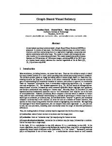
Figure 2: Encoding image content (from left to right): Input image. Occupancy distribution of bins within color cube. Occupied bins O, initial and final encoding vectors E. Encoded image by assigning closest encoding vector per pixel.

3. Encoding Based Saliency

information is lost. Therefore, we propose an efficient approximation by lower-dimensional joint distributions using encoding vectors.

3.1. A Bayesian Saliency Formulation Following the Gestalt principle for figure-ground segregation, we are searching for surrounded regions as they are more likely to be perceived as salient areas [20]. In other words, we analyze the contrast between the distribution of an image region (e.g. rectangle) with its surrounding border. Similar to [17, 21], we first define a Bayesian salience measurement. To distinguish salient foreground pixels x ∈ F from surrounding background pixels, we employ a histogram based Bayes classifier on the input image I. Therefore, let HΩ (b) denote the b-th bin of the nonnormalized histogram H computed over the region Ω ∈ I. Furthermore, let bx denote the bin b assigned to the color components of I(x). Given a rectangular object region F and its surrounding region S (see Figure 1), we apply Bayes rule to obtain the foreground likelihood at location x as P (bx |x ∈ F ) P (x ∈ F ) P (x ∈ F|F, S, bx ) ≈ P . P (bx |x ∈ Ω) P (x ∈ Ω)

(1)

Ω∈{F,S}

We estimate the likelihood terms by color histograms, i.e. P (bx |x ∈ F ) ≈ HF (bx )/|F | and P (bx |x ∈ S) ≈ HS (bx )/|S|, where |·| denotes the cardinality. Additionally, the prior probability can be approximated as P (x ∈ F ) ≈ |F |/(|F | + |S|). Then, Eq. (1) simplifies to ( HF (bx ) if I(x) ∈ I(F ∪S) P (x ∈ F|F, S, bx ) = HF (bx )+HS (bx ) (2) 0.5 otherwise, where unseen pixel values are assigned the maximum entropy prior of 0.5. This discriminative model already allows us to distinguish foreground and background pixels locally. However, modeling the joint distribution of color values, represented by 10 bins per channel, within a histogram based representation as described above, would lead to 103 dimensional features to describe solely color information. Assuming independence between channels as in [21] would simplify the problem to 3 × 10 dimensions and would allow using efficient structures (e.g. integral histograms), but

3.2. Estimating Joint Distributions via Encoding Analyzing the content of single images or video frames yields in general an exponential distribution of occupied bins as shown in Figure 2. The majority of image content is represented by a small number of occupied bins within a 10 × 10 × 10 color cube representing the joint distribution, namely 33 bins cover 95% of the data samples in this example, while overall only 150 of 1000 possible bins are occupied (blue dots). Taking only the bins covering 95% (red dots) has two major weaknesses. First, their spatial distribution is not efficiently covering the occupied volume within the color cube, leading to approximation artifacts. Second, the threshold for 95% may increase the number of taken bins to more than 80 as stated in [5], limiting the applicability for efficient sliding window computations. Instead, we propose to represent the image content by a fixed number of encoding vectors. Let O ∈ Ro×d represent all occupied bins and E ∈ RN e×d the set of N e encoding vectors where N e ≤ |O|. We initialize E with the N e most occupied bins (i.e. red dots in Figure 2) and perform kmeans clustering to optimize for the spatial distribution of encoding vectors as arg min E

Ne X X

2

ko − ei k ,

(3)

i=1 o∈E(i)

where E(i) denotes the set of bins o clustered to the encoding vector ei . The number of encoding vectors is set to the number of occupied bins covering 95% image pixels if this number is smaller than a maximum N e. The final encoding vectors E, visualized with green dots, and the resulting encoded image with N e = 30 are also shown in Figure 2. Homogenous regions are encoded by a small number of codes, while detailed structures are preserved. Please note that the final encoding vectors are not required to correspond to bins in the color cube. To further relax

the hard binning decisions of color histograms, we perform a weighted encoding over the nearest encoding vectors of each element in O. When creating the integral histogram structure H (for simplicity we use the same notation as for histograms in Section 3.1), the entry for the k-th bin at pixel position x is computed by

H (x, k) =

 1 −

ko(x)−ek k2 P ko(x)−ej k2

if k ∈ N (o(x), E) (4)

j∈N (o(x),E)



0

otherwise,

where H ∈ Rh×w×N e and o(x) defines the occupied bin I(x) belongs to. The set of j encoding vectors nearest to o(x) is given by N (o(x), E). Compared to other saliency approaches based on segmenting or clustering images, our overall process is very efficient as number and dimensionality of vectors in O is relatively small (in general around 200 occupied bins have to be considered) compared to pixels per image (above 200k), and converges in a fraction of a second. In addition, all operations for mapping I(x) to H(x) can be efficiently performed using lookup-tables. The result of such soft-encoded histogram structures is visualized in Figure 2. Next, we discuss how to enforce the Gestalt principle of figure-ground segregation on local and global scales.

3.3. Saliency Map Computation Once the integral histogram structure of encoding vectors is created as described above, we can efficiently compute the local foreground saliency likelihood Φ(x) for each pixel by applying Eq. (2) in a sliding window over the image. To this end, the inner region F of size [σi × σi ] is surrounded by the [2σi × 2σi ] region S. Then, the following processing steps are performed on each scale σi . First, we iterate over the image with a step size of σ4i to ensure that the foreground likelihood for each pixel is estimated against different local neighboring constellations. Within each calculation, the foreground likelihood values of all pixels inside F are set. The final likelihood value for Φi (x) is obtained as the maximum value over all neighborhood constellations. Second, following our original motivation by Gestalt theory, the foreground map for scale i should contain highlighted areas for salient regions of size σi or smaller. In contrast, a region significantly larger than σi would have likelihood values Φi (x) ≤ 0.5 for x ∈ F . Therefore, the figure-ground segregation can be easily controlled after computing the foreground likelihood map by applying a box filter of size [σi × σi ], and setting Φi (x) to ¯ i (x) ≤ 0.5. Fizero if the average foreground likelihood Φ nally, local foreground maps Φi (x) are filtered by a Gaussian with kernel width σ4i . The local foreground maps of individual scales are linearly combined to one local foreground saliency map ΦL , which is L∞ normalized.

Besides these locally computed foreground maps, global estimation of salient parts also offers valuable information. In particular, we observed that videos or images with global camera motion or homogenous background regions benefit from such global information. To compute the global foreground likelihood map ΦG , we set S to the image border (typically 10–20% of the image dimensions) and F is the non-overlapping center part of the image. The resulting foreground saliency map ΦG is Gaussian filtered and L∞ normalized.

3.4. Processing Motion Information Studying related approaches for video saliency we found that optical flow information is incorporated in general with less care than appearance information. Measurements like pure flow magnitude [21, 23], motion gradients [27] or simple attributes like velocity, acceleration or average motion [33] are treated independently, respectively without motion orientation information. However, considering the pseudo-color optical flow representation in Figure 1, we can directly observe that magnitude or simple attributes are prone to fail if large global camera motion is present and motion gradients create a noisy response. On the other hand, we observe a very discriminative visual representation of the scene context, which motivated us to have a closer look on the creation of such pseudo-color representations for optical flow. Following [24], the motion components for horizontal and vertical directions given in U (x) and V (x) are mapped to a color wheel representing the transitions and relations between the psychological primaries red, yellow, green, and blue. The color wheel, also known as Munsell color system, arranges colors such that opposite colors (at opposite ends of the spectrum, e.g. red and blue) are most distant to each other on the wheel. Similarly, we want to represent opposite motion directions most distant to each other. Therefore, we directly apply our approach represented in Sections 3.2 and 3.3 on the pseudo-color motion representation. To this end, we compute the magnitude M (x) and oriˆ (x) and Vˆ (x), which are the optical flow entation Θ(x) of U components normalized by the maximum magnitude of the corresponding frame. The orientation Θ(x) defines the hue value in the color wheel, while saturation is controlled by M (x). Applying precomputed color wheel lookup tables, we directly generate a three dimensional pseudo-color image taken as input for our motion saliency pipeline. Similar to the appearance likelihood maps ΦAL and ΦAG this yields the motion-based local ΦM L and global ΦM G likelihood maps. Although relatively simple, experimental evaluations show the beneficial behavior of this motion representation compared to related approaches discussed at the beginning of this section.

3.5. Adaptive Saliency Combination Given the above described steps, we generate up to four foreground maps for local and global estimation of appearance (i.e. ΦAL and ΦAG ) and motion (i.e. ΦM L and ΦM G ) saliency. Previous works either directly merged cues [27] or performed coarse global measurements like pseudo-invariance [31] without incorporating the spatial distribution of maps. In contrast, we approximate the uncertainty within our individual saliency maps, by computing weighted covariance matrices of each map. This allows us to cope with inaccuracies of individual maps. A weighted covariance for saliency map Φj is given as: P P  Φj (x,y)(¯ x−¯ µx )(¯ y −¯ µy )  Φj (x,y)(¯ x−¯ µx ) x,y∈I

x,y∈I

P  Φ (x,y)  P x,y∈I j Σj = Φj (x,y)(¯x−¯µx )(¯y−¯µy ) x,y∈I P

Φj (x,y)

x,y∈I

P

Φj (x,y)

Px,y∈I Φj (x,y)(¯ y −¯ µy ) P Φj (x,y)

x,y∈I

  , 

x,y∈I

(5) where x ¯, y¯ denote normalized image coordinates to avoid bias for rectangular images and µ ¯x , µ ¯y are the corresponding mean coordinates. Taking Σu as the baseline covariance of an unweighted uniform distribution, the reliability or weighting score for map j is computed as ωj = 1 −

det(Σj ) , det(Σu )

where

X j

ωj = 1.

(6)

Then, P the final saliency map can be directly obtained by Φ = j ωj Φj . In the following, we denote our encoding based saliency approach EBS for unweighted linear combination of local saliency maps. In contrast, EBSL uses the proposed weighted combination of solely local and EBSG the weighted combination of all available (local & global) likelihood maps.

4. Experiments In the following, we perform various experiments for both video saliency and object saliency tasks. First, we demonstrate the favorable performance of our approach for challenging video saliency tasks using the Weizmann [7] and UCF Sports [22] activity datasets. Second, we compare EBS to related saliency approaches and evaluate the influence of parameter settings on the widely used ASD [1] salient object dataset. Further results may be found within the supplementary material. As ground-truth annotations are given in different formats (i.e. coarse bounding boxes, detailed binary segmentation or eye-fixation maps), we apply the following metrics correspondingly. If ground-truth segmentations are available, we compute precision/recall values as well as the area under curve (AUC) by varying thresholds to binarized saliency map and measure the overlap with the ground-truth segmentation. For experiments where solely bounding box

annotations are available, we add spanning bounding boxes to the binarized saliency map before computing the scores (denoted AUC-box, please see supplementary material for more details). For given eye-gaze ground-truth data, we measure the exactness of the saliency maps by computing the normalized cross correlation (NCC). For all benchmark comparisons we use code or precomputed results published by the corresponding authors, except for [27] which we reimplemented according to the paper (without 3D MRF smoothing which could be optionally applied to all methods).

4.1. Saliency for Activity Localization Recent evaluation of video saliency methods by [33] on the Weizmann activity dataset [7] has shown the superior performance of solely color-based methods. For completeness, we compare against their results within the supplementary material, but based on our findings in this experiment, we further evaluate on a more selective activity dataset, namely the UCF Sports dataset [22], which is a collection of low-quality television broadcasts, containing 150 videos of various sports. This dataset depicts challenging scenarios including camera motion, cluttered backgrounds, and non-rigid object deformations. Furthermore, it provides ground-truth bounding box annotations for all activities. In addition, [18] captured eye-gaze data from 16 subjects, which allows to compare saliency results with these human attention maps given as probability density functions (see Figure 5). This makes the dataset well suited for benchmarking our EBS with other video saliency methods. For comparison, we apply all top performing methods from [33] and additionally include [27]. Furthermore, we use the objectness detector of [2], as previously applied for weakly supervised training of activity detectors on UCF Sports by [26]. We follow their parametrization and take the top 100 boxes returned by the objectness detector to create a max-normalized saliency map per frame. For completeness, we quote NCC scores from [25] for supervised eye-gaze estimation trained and evaluated via cross-validation on UCF Sports. Please note that all saliency methods, others and the proposed EBS, are fully unsupervised and require no training. The objectness detector [2] is trained on the PASCAL object detection benchmark dataset. For a distinct evaluation we split the videos into two sets, namely static and dynamic, where the first contains activities with less severe background clutter or motion like golfing, kicking, lifting, swinging, and walking. The second set consists of activities with strong camera motion, clutter, and deformable objects, such as diving, horse-riding, skating, swing on bar, and running. As can be seen from the resulting recall/precision curves in Figure 3, all methods perform better on the static videos than on the dynamic ones. The most significant performance decrease between static and

AUC AUC-box NCC

Eye-gaze 0.61 0.77 1.00

[11] 0.44 0.51 0.36

[2] 0.52 0.52 0.33

[27] 0.48 0.65 0.33

[33] 0.47 0.61 0.37

[21] 0.43 0.54 0.32

DJS 0.64 0.73 0.43

EBS 0.58 0.68 0.47

EBSL 0.60 0.70 0.45

EBSG 0.66 0.73 0.47

[25] − − 0.36*

[18] − − 0.46*

Table 1: Average AUC, AUC-box and NCC scores over all UCF Sports videos.* NCC scores for supervised methods trained on UCF sports published by [25].

static

1

1

0.9

0.9

0.8

0.8

0.7

0.7

0.6

0.6

precision

precision

static (box)

0.5 0.4

0.5 0.4

0.3

0.3 eye−gaze Alexe"10 Rathu"10 Zhou"14

0.2 0.1

Sultani"14 EBS EBSG EBSL

0.2 0.1

0

0 0

0.2

0.4

0.6

0.8

1

0

0.2

0.4

recall

0.6

0.8

1

0.8

1

recall

(a)

(b)

dynamic (box)

dynamic

1

1

0.9

0.9

0.8

0.8

0.7

0.7

0.6

0.6

precision

precision

dynamic videos can be observed for [33] which is the topperforming method on the simpler Weizmann experiments. On the contrary, our EBS versions show almost no degradation when switching from simpler static to more complex dynamic scenes. Furthermore, we observe a larger gap between using solely local EBSL and incorporating global information within EBSG on the dynamic videos. This can be explained by our optical flow representation which acts as a kind of global motion compensation when computing the global motion saliency. In particular, our flow representation performs favorably compared to [21, 27, 33] which rely on simple motion magnitude. Overall, all compared methods benefit from the box prior when evaluating recall and precision, as it compensates for coarse annotations and supports sparse saliency maps as generated by [27, 33]. Another interesting point to see is that human eye-gaze does not perform superior when evaluated against bounding box annotations, especially considering the simpler static videos. After having a closer look on the results, it can be seen that human fixations are focused on faces if the image resolution is sufficiently high and the image context is less demanding. On the other hand, for low resolution videos or rapidly changing actions the fixations are distributed over the whole person (see Figure 5). This is fully consistent with previous findings of [13], but questioning the general applicability of human eye-gaze as supervision for training activity detectors, as e.g. in [25]. Table 1 summarizes the results over all UCF Sports videos. As can be seen, our EBS methods perform favorably compared to other video saliency methods and on par with previously proposed supervised methods trained and tested on UCF Sports. DJS depicts the results for directly modeling the joint distribution of color and motion channels for saliency estimation, as described in Section 3.1. As this incorporates a 1000-dimensional histogram when working with 10 bins per color channel, we cannot perform optimizations like integral histograms as described in Section 3.2, therefore leading to inferior run-times, while our MATLAB implementation of EBS is comparable to other benchmarked methods and still has potential for optimization. The difference between DJS and EBS is the loss of encoding up to several hundred color values per image with 30 or less encoding vectors. But this loss can be captured by our adaptive weighting of individual saliency cues within EBSL and EBSG.

0.5 0.4

0.5 0.4

0.3

0.3 eye−gaze Alexe"10 Rathu"10 Zhou"14

0.2 0.1

Sultani"14 EBS EBSG EBSL

0.2 0.1

0

0 0

0.2

0.4

0.6

0.8

1

0

recall

(c)

0.2

0.4

0.6 recall

(d)

Figure 3: Average recall-precision plots of various saliency methods on UCF-sports dataset. Results over static videos with (a) or without (b) box prior. Results over dynamic videos (c), (d). The dynamic subset contains much more challenging videos including moving cameras, cluttered background and non-rigid object deformations during actions. See text for further discussion.

4.2. Salient Object Detection One of the most similar tasks to localizing activities in videos is salient object detection in still images. Both tasks have the goal of finding eponymous regions in the data. Altough the focus of our work is on saliency estimation for activity videos, EBS can easily be applied to standard image saliency tasks by switching off the motion components. Many models and datasets have been proposed in the image domain (see e.g. [3, 4] for a review). In particular, we use the ASD dataset [1], which comprises 1000 im-

1 https://lrs.icg.tugraz.at/

using RGB or Lab color channels. But we see a strong improvement from applying our methods on distributions following the independency assumption between channels, similar to [21] denoted as (independent Rgb, Lab ), to our approximated joint distributions in EBSG. state−of−the−art (no segmentation)

1

1

0.9

0.9

0.8

0.8

0.7

0.7

0.6

0.6

precision

precision

state−of−the−art (with segmentation)

0.5 0.4 GSGD GSSP Hsal BMS RC EBSG EBSGR

0.3 0.2 0.1

0.5 0.4 0.3 HC FT HFT EBSG EBSGR

0.2 0.1

0

0 0

0.2

0.4

0.6

0.8

1

0

0.2

0.4

recall

0.6

0.8

1

recall

(a)

(b)

non−centered objects

color spaces

1

1

0.9

0.9

0.8

0.8

0.7

0.7

0.6

0.6

precision

precision

ages with ground-truth segmentation masks. We benchmark against recent state-of-the-art approaches, such as FT [1], HFT [14], BMS [32], Hsal [30], GSGD & GSSP [29], and RC & HC [5]. A comparison with the state-of-the-art in salient object segmentation is shown in Figure 4. To utilize the full potential of our encoding information, we added a postprocessing step which exploits the soft segmentation of the image by assigning each pixel to a number of encoding vectors, as described in Section 3.2. As depicted in Figure 2, encoding vector assignment creates a data dependent over-segmentation. EBSGR uses this over-segmentation and propagates high EBSG saliency values within these segments, leading to less smooth and more object related saliency map results. More information is given in the supplementary and online1 . EBSG and EBSGR perform better or equal than approaches without explicit segmentation steps, i.e. [1, 5, 14]. The top-performers on the other hand enforce segmentation-consistent results [30] or pose additional assumptions, e.g. the object must not be connected to the image border [29, 32]. Both constraints are particularly beneficial for the ASD dataset, but questioned by the recent analysis in [15]. Therefore, we evaluate the impact of the latter object-center prior by cropping images of the ASD dataset such that salient objects are located near the borders. We compare our EBSG against the top performing BMS [32] using two cropping levels: First, salient objects touch the closest image border and second, intersect the closest border by 5 pixel. As shown in Figure 4c, the robustness of BMS decreases drastically while EBSG stays almost constant within the first test and decreases slightly for severe out of center objects. A visual comparison on exemplar figures can be found in the supplementary material. Within all experiments we applied 7 local scales between 1 , . . . , 12 ] min (width, height) of each individual σi = [ 10 test image. Post-processing at each scale level is performed as described in Section 3.3. We fixed the number of bins per color channel to 10 and the maximum number of encoding vectors N e to 30 within all experiments, as the average number of encoding vectors chosen by EBS lies below 30 for both RGB and CIE Lab (see Section 3.2). Finally, we evaluate the influence of taking RGB or CIE Lab color spaces. Further, we evaluate the benefit of joint modeling feature channel probabilities within our EBS compared to saliency estimation with independent color channel probabilities as previously done by e.g. [21, 31]. Results in Figure 4d show that increasing the number of maximally available encoding bins N e from 30 to 60 does not improve results because, as mentioned above, the number of encoding vectors is set to the number of occupied bins responsible for 95% (if this number is smaller than the maximum N e). The results do not show considerable differences between EBSG

0.5 0.4

0.5 0.4

0.3

independent Rgb independent Lab EBSG (rgb,60) EBSG (lab,60) EBSG (rgb,30) EBSG (lab,30)

0.3 BMS border BMS intersect EBSG border EBSG intersect

0.2 0.1

0.2 0.1

0 0

0.2

0.4

0.6 recall

(c)

0.8

1

0

0

0.2

0.4

0.6 recall

0.8

1

(d)

Figure 4: (a) comparison of EBSG and EBSGR (b) to stateof-the-art in salient object detection on ASD dataset. (c) Results of top performing BMS decrease drastically if objects are placed at image borders (see text for more details). (d) Our EBSG performs favorable compared to independence assumption for color channels.

5. Conclusion We proposed a novel saliency detection method inspired by Gestalt theory. Analyzing the image or video context respectively, we create encoding vectors to approximate the joint distribution of feature channels. This low-dimensional representation allows to efficiently estimate local saliency scores by applying e.g. integral histograms. Implicitly enforcing figure-ground segregation on individual scales allows us to preserve salient regions of various sizes. Our robust reliability measurement allows for dynamically merging individual saliency maps, leading to excellent results on challenging video sequences with cluttered background and camera motion, as well as salient object detection in images. We believe that further statistical measurements

Figure 5: Exemplar of video saliency results on UCF sports. Top row: Input images with ground-truth annotations. Second row: Eye-gaze tracking results collected by [18]. From row three to bottom: Our proposed method (EBSG), objectness detector [2], color saliency[11], video saliency methods [21] and [33]. See text for detailed discussion. for saliency reliability and incorporation of additional topdown saliency maps could further augment our approach.

Acknowledgments. This work was supported by the Austrian Science Foundation (FWF) under the project Advanced Learning for Tracking and Detection (I535-N23).

References [1] R. Achanta, S. Hemami, F. Estrada, and S. S¨usstrunk. Frequency-tuned Salient Region Detection. In CVPR, 2009. 2, 5, 6, 7 [2] B. Alexe, T. Deselaers, and V. Ferrari. What is an object? In CVPR, 2010. 5, 6, 8 [3] A. Borji, D. Sihite, and L. Itti. Salient Object Detection: A Benchmark. In ECCV, 2012. 2, 6 [4] Z. Bylinskii, T. Judd, F. Durand, A. Oliva, and A. Torralba. MIT Saliency Benchmark. http://saliency.mit.edu/. 6 [5] M.-M. Cheng, N. J. Mitra, X. Huang, P. H. S. Torr, and S.-M. Hu. Global contrast based salient region detection. In CVPR, 2011. 2, 3, 7 [6] X. Cui, Q. Liu, and D. Metaxas. Temporal spectral residual: fast motion saliency detection. In ACM MM, 2009. 2 [7] L. Gorelick, M. Blank, E. Shechtman, M. Irani, and R. Basri. Actions as Space-Time Shapes. PAMI, 29(12):2247–2253, 2007. 5 [8] C. Guo, Q. Ma, and L. Zhang. Spatio-temporal Saliency detection using phase spectrum of quaternion fourier transform. In CVPR, 2008. 2 [9] J. Harel, C. Koch, and P. Perona. Graph-based Visual Saliency. In NIPS, 2006. 2 [10] L. Itti, C. Koch, and E. Niebur. A model of saliency-based visual attention for rapid scene analysis. PAMI, 20(11):1254– 1259, 1998. 2 [11] H. Jiang, J. Wang, Z. Yuan, N. Zheng, and S. Li. Automatic Salient Object Segmentation Based on Context and Shape Prior. In BMVC, 2011. 6, 8 [12] G. Johansson. Visual perception of biological motion and a model for its analysis. Perception & Psychophysics, 14(2):201–211, 1973. 1 [13] T. Judd, K. Ehinger, F. Durand, and A. Torralba. Learning to Predict Where Humans Look. In ICCV, 2009. 1, 6 [14] J. Li, Levine, M.D., X. An, X. Xu, and H. He. Visual Saliency Based on Scale-Space Analysis in the Frequency Domain. PAMI, 35(4):996–1010, 2013. 2, 7 [15] Y. Li, X. Hou, C. Koch, J. Rehg, and A. L. Yuille. The secrets of Salient Object Segmentation. In CVPR, 2014. 7 [16] T. Liu, J. Sun, N.-N. Zheng, X. Tang, and H.-Y. Shum. Learning to Detect A Salient Object. In CVPR, 2007. 2 [17] V. Mahadevan and N. Vasconcelos. Spatiotemporal Saliency in Dynamic Scenes. PAMI, 32(1):171–177, 2010. 3 [18] S. Mathe and C. Sminchisescu. Dynamic Eye Movement Dataset and Learnt Saliency Models for Visual Action Recognition. In ECCV, 2012. 2, 5, 6, 8 [19] P. Mital, T. Smith, R. Hill, and J. Henderson. Clustering of Gaze During Dynamic Scene Viewing is Predicted by Motion. Cognitive Computation, 3(1):5–24, 2011. 1 [20] S. E. Palmer. Vision Science, Photons to Phenomenology. MIT Press, 1999. 3 [21] E. Rahtu, J. Kannala, M. Salo, and J. Heikkil¨a. Segmenting Salient Objects from Images and Videos. In ECCV, 2010. 1, 2, 3, 4, 6, 7, 8 [22] M. D. Rodriguez, J. Ahmed, and M. Shah. Action MACH - A Spatio-temporal Maximum Average Correlation Height Filter for Action Recognition. In CVPR, 2008. 5

[23] D. Rudoy, D. B. Goldman, E. Shechtman, and L. ZelnikManor. Learning Video Saliency from Human Gaze Using Candidate Selection. In CVPR, 2013. 2, 4 [24] D. Scharstein. Middlebury Optical Flow Benchmark. http://vision.middlebury.edu/flow/. 4 [25] N. Shapovalova, M. Raptis, L. Sigal, and G. Mori. Action is in the Eye of the beholder: Eye-gaze Driven Model for Spatio-Temporal Action Localization. In NIPS, 2013. 2, 5, 6 [26] N. Shapovalova, A. Vahdat, K. Cannons, T. Lan, and G. Mori. Similarity Constrained Latent Support Vector Machine: An Application to Weakly Supervised Action Classification. In ECCV, 2012. 5 [27] W. Sultani and I. Saleemi. Human Action Recognition across Datasets by Foreground-weighted Histogram Decomposition. In CVPR, 2014. 2, 4, 5, 6 [28] E. Vig, M. Dorr, and D. Cox. Large-Scale Optimization of Hierarchical Features for Saliency Prediction in Natural Images. In CVPR, 2014. 1, 2 [29] Y. Wei, F. Wen, W. Zhu, and J. Sun. Geodesic Saliency Using Background Priors. In ECCV, 2012. 2, 7 [30] Q. Yan, L. Xu, J. Shi, and J. Jia. Hierarchical Saliency Detection. In CVPR, 2013. 2, 7 [31] Y. Zhai and M. Shah. Visual Attention Detection in Video Sequences Using Spatiotemporal Cues. In ACM MM, 2006. 2, 5, 7 [32] J. Zhang and S. Sclaroff. Saliency Detection: A Boolean Map Approach. In ICCV, 2013. 1, 2, 7 [33] F. Zhou, S. B. Kang, and M. F. Cohen. Time-Mapping using Space-Time Saliency. In CVPR, 2014. 2, 4, 5, 6, 8