Lesion detection using Gabor-based saliency field

Lesion detection using Gabor-based saliency field mapping Marc Macenkoa , Rutao Luoa , Mehmet Celenka , Limin Maa , and Qiang Zhoub a School

of Electrical Engineering and Computer Science, Ohio Univ., Athens, OH 45701, USA b Chrontel Inc., San Jose, CA 95131 ABSTRACT

In this paper, we present a method that detects lesions in two-dimensional (2D) cross-sectional brain images. By calculating the major and minor axes of the brain, we calculate an estimate of the background, without any a priori information, to use in inverse filtering. Shape saliency computed by a Gabor filter bank is used to further refine the results of the inverse filtering. The proposed algorithm was tested on different images of ”The Whole Brain Atlas” database.8 The experimental results have produced 93% classification accuracy in processing 100 arbitrary images, representing different kinds of brain lesion. Keywords: brain lesion, background estimation, Gabor-filter

1. INTRODUCTION Detection of abnormal, anatomical brain structures with their location and orientation is an extremely important task in the diagnosis stage and in the planning and analysis of various treatments including radiation therapy and surgery.1, 3, 4 Because of this importance, accurate lesion diagnosis is a highly active area of study. In recent years, significant research effort has been devoted to the development of medical-imaging systems for an early detection of brain anomalies. For example, in1 the authors utilize statistical analysis to track the changes of brain lesions across the temporal dimension to assess treatment outcomes. A deformable model is employed in3 to accurately segment volumetric heart data to aid in visualization. In,4 the authors use maximal likelihood estimation in conjunction with deformable models to accurately segment tumors in functional images of mice. In our research, lesion detection is carried out by combining the output of our spectral subtraction method with the shape saliency produced by a bank of Gabor filters. The result is a belief map that contains a value between zero and one for each pixel. A value of zero indicates the certain belief that the pixel is ordinary. A value of one corresponds to a certain belief that the pixel belongs to a region of interest. A similar approach was taken in.10 We use a priori information about the overall shape of the brain in order to estimate the spectrum of the background and about the shape of lesions to guide the thresholding of the belief map. An image model is devised in such a way that it captures the interrelation among the region of interest (ROI) and background with the inclusion of a blurring function and additive noise in the analytical model.2, 4–6 The results show that the proposed approach achieves more accurate segmentation results than the use of morphological watershed segmentation as a stand alone processing tool and of our improved algorithm that requires healthy slices. The remaining part of this paper is organized as follows. In section 2, a description of the overall approach is presented in detail. Section 3 is devoted to experimental results and performance assessment of the approach developed in this research. Conclusions and further research topics are given at the end. Further author information: (Send correspondence to Mehmet Celenk) Marc Macenko: E-mail: [email protected] Rutao Luo: E-mail: [email protected] Mehmet Celenk: E-mail: [email protected], Telephone: 1 740 593 1581 Limin Ma: E-mail: [email protected] Qiang Zhou: E-mail: [email protected]

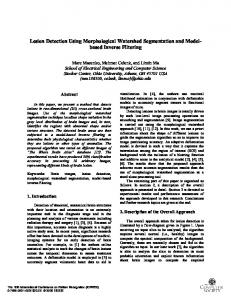
2. DESCRIPTION OF THE OVERALL APPROACH The overall approach taken for lesion detection is illustrated by a flow-diagram given in Figure 1. Upon receiving an input slice to be analyzed, the algorithm computes the major and minor axes of the brain image to calculate the spectral composition of the background. The orientation of these axes is calculated from the modified principle component analysis of the image (see Figure 2).7 Once the spectral characteristics of the background and the observed signal (i.e., the slice to be analyzed) have been computed, frequency domain subtraction is employed to estimate the desired signal, that is, the spectrum of the lesions and/or other abnormalities. The spectrally estimated 2D signal is then converted to the spatial domain to find the abnormalities present in the brain. Sections 2.1 and 2.2 provide further discussion on this process. Next, the shape saliency of the input image is computed by a bank of Gabor filters each with a different orientation. Section 2.3 includes further discussion. Section 2.4 contains the details of the process of thresholding the belief map and eliminating erroneous results.

Figure 1. Block diagram representation of the lesion detection system.

2.1. Adaptive Deformation Modeling Once regions of interest (ROI) are delineated, an adaptive deformation modeling algorithm is driven to find the contour and size of each lesion. In 2D cross sectional representation, our deformable model is essentially a flat planar region of the volumetric lesion whose boundary can be described by a circular or ellipsoid type analytical expression. It is allowed to deform in an arbitrary way with penalties associated with random motion. Blurring is taken into account and Gaussian white noise is added to the deformable template to aid in matching. The region is labeled appropriately depending on which model provides the lowest cost match based on warping to fit the object. The model adopted herein can be defined analytically by2 f (s, t) = [v(s, t) + b(s, t)] ∗ g(s, t) + n(s, t)

(1)

Here, f (s, t) is the observed image, v(s, t) is the deformable model, b(s, t) is the background, g(s, t) is the known blurring point-spread function, n(s, t) is the additive Gaussian white noise, s is the 2D spatial domain variable (x,y)-coordinates of a point, and t denotes cross-sectional slice index in the 3D space.

2.2. Spectral Subtraction Method To solve for the target ROI v(s,t) in Equation (1), we take the Fourier transform of f(s,t). This results in F (w, t) = [V (w, t) + B(w, t)] · G(w, t) + N (w, t)

(2)

Figure 2. A sample calculation of the major axes.

where, F (w, t), V (w, t), B(w, t), G(w, t), and N (w, t) are the 2D spatial-domain Fourier transforms of f (s, t), v(s, t), b(s, t), g(s, t), and n(s, t), and w is the frequency domain variable (wx , wy ) corresponding to the variations in the (x,y)-spatial plane coordinates, respectively. After some arithmetic manipulation, we arrive at the inverse filtering relation of the form V (w, t) = {[F (w, t) − N (w, t)]/G(w, t)} − B(w, t)

(3)

If there is no blurring (i.e., G(w,t) = 1) and noise has already been eliminated (i.e., N(w,t) = 0) via Weiner or Gaussian filtering, we are left with the simplified, yet powerful, formulation which is given by V (w, t) = F (w, t) − B(w, t)

(4)

This lends itself directly to the spectral subtraction method that is widely used to reduce the noise in speech or other audio signals (see Figure 3).9

2.3. The Multiple Channel Filter Model and Shape Saliency Multi-channel filtering is a multi-resolution decomposition process. The set of Gabor functions is one well-know class of functions that is able to achieve both spatial and spatial-frequency localization. This kind of wavelet has been extensively used in shape detection due to the ability to tune a Gabor filter to a specific spatial frequency and orientation, and achieve both localization in the spatial and the spatial frequency domains.14–17 2.3.1. Gabor Channel Filter In this section, the basis properties of the 2-D Gabor filter are described. The complex 2-D Gabor function is defined by h(x, y) = g 0 (x, y)ej(ωx x+ωy y) (5) where g 0 (x, y) =

x0 y 0 1 − x2 +y2 1 2 g( , ), g(x, y) = e 2 λσ λσ σ 2π

(6)

x0 = x cos θ + y sin θ, y 0 = −x sin θ + y cos θ

(7)

That is, g 0 (x, y) is a version of the Gaussian g(x, y) that is spatially scaled and rotated by θ. The parameter σ is the special scaling, which controls the width of the filter impulse response, and λ defines the aspect ratio of the filter, which determines the directionality of the filter. The orientation angle θ is usually chosen to be equal to the direction of the filter’s center circular frequency12 θ = tan−1

ωy ωx

(8)

Figure 4 depicts the magnitude of the complex Gabor filter for λ=0.3, σ=1, θ=0. Let σx = λσ, σy = σ, we can rewrite the equation (6) as g 0 (x, y) =

1 x0 y 0 g( , ) σx σy σx σy

Figure 3. Result of spectral subtraction method using estimated background for the same input as in Figure 1.

Figure 4. Plot of the magnitude of the point spread function of a Gabor filter.

(9)

In the spatial-frequency domain, the Gabor filter becomes a Gaussian shifted to the location of the modulating frequency. The equation of the 2-D frequency response of the filter is given by H(u, v) = e−2π

2

2 [σx (u−u0 )2 +σy2 (v−v0 )2 ]

(10)

The frequency u0 , v0 and the rotation angle θ define the center location of the filter. By tuning u0 , v0 and θ to different center locations we can create multiple filters that cover the spatial frequency domain. 2.3.2. Filter Bank Design The process of shape detection using multi-channel filtering can be outlined as follows: 1)Design the appropriate filter bank; 2)Decompose the input image using the filter bank; 3)Detect the shapes that are sought. As mentioned above, specification of the filter set properties involves choosing a set of frequencies and orientations that will cover the spatial-frequency space, and capture shape information as much as possible. In this work, we used 16 Gabor filters to compose the multiple channel filter bank. We need to tune the following four parameters for each filter: σx : The variance along x , σy : The variance along y q ω: The filter’s center circular frequency ω = ωx2 + ωy2 θ: The orientation angle Here, we set the same σx , σy , and ω for each filter: σx =1 , σy =1 , ω=0.2 The sixteen values listed below for the parameter θ were selected to properly capture the shape information. 6π 5π 4π 3π 2π 1π 1π 2π 3π 4π 5π 6π 7π 8π θ = {− 7π 16 , − 16 , − 16 , − 16 , − 16 , − 16 , − 16 , 0, 16 , 16 , 16 , 16 , 16 , 16 , 16 , 16 }

2.3.3. Shape Detection Many computer vision applications, such as object recognition and active vision, could function more reliably and effectively if objects of interest were isolated from their background. With no knowledge, it is a difficult task to determine which image regions are interesting. For each problem, region saliency is defined in terms of features that capture essential visual or perceptual attributes such as color, texture, and shape characteristics. In this way, an image is mapped onto the appropriate feature space so that salient regions can be identified more easily.13 Here, we propose a simple ROI detection algorithm directly working on grey-level images. The saliency of each pixel is measured by the influence of wavelet coefficients variance saliency, with proper enforcement of the smoothness in the neighborhood. Mathematically it can be defined as the functional ZZ s = argmin [α(s(x, y) − fw (x, y))2 + β(g(||∇s(x, y)||))] dxdy (11) where s(x, y) represents the saliency of the pixel at location (x, y). The parameter α controls the interrelation between the wavelet saliency and neighborhood variance saliency while β determines the smoothness of the saliency field map. Here, g is the truncated quadratic potential function.10 In Equation (13), the wavelet coefficients variance based saliency fw (x, y) is defined as an N-dimensional sigmoid function by N Y

1

(12) var(x,y)n (rn + e varave ) where N is the total number of filters; var(x, y)n is the local variance for each channel of the wavelet transform of the original gray-level image at location (x,y); the weights of the different channels are controlled by the variable constant coefficients rn , which are all set to be 0.5 for our experiments; The variable constants varave , are the mean values of the local variances of the corresponding wavelet channels. The resulting saliency is normalized so that the neighborhood saliency ranges from zero to one. Conceptually, for an image containing objects and background, sometimes the objects are focused and the background is not. Therefore, the high frequency channels of the wavelet transform have large variance in coefficients for focused regions. As shown in Figure 5, the brighter the value of a pixel, the higher the wavelet-based saliency value. fw =

n=1

−

2.4. Belief Map Thresholding The belief map generated from the inverse filtering and shape saliency contains a value between zero and one for each pixel of the input image. A value of zero indicates the certain belief that the pixel is ordinary. A value of one corresponds to a certain belief that the pixel belongs to a region of interest (see Figure 6). Experimentation has shown that a threshold value of 0.5 successfully avoids erroneous regions while capturing most of the area belonging to the lesion. Holes in the regions resulting from the thresholding are filled in to support continuity of detected areas.

Figure 5. Shape saliency calculated for the same input image as the previous examples.

Figure 6. Belief map resulting from the combination of the spectral subtraction and the shape saliency on the same input as in Figure 1.

3. EXPERIMENTAL RESULTS This result is again thresholded, removing objects that are either too small or too eccentric. Here, eccentricity of an area is defined as the ratio of the distance between the foci of the ellipse that has the same second moments of the area and the length of its major axis.11 This takes on values from zero (corresponding to a circular area) to one (corresponding to a line segment with unit width). The eccentricity constraint takes into account the a priori knowledge that lesions and other anomalies tend to be close to elliptical (see Figure 7).

Because the standard mode of 3D medical image acquisition is that of obtaining many 2D slices and combining these into a 3D volume, particular 2D slices were examined in this study. The algorithm was run on sample images of the database ”The Whole Brain Atlas”8 (see Figures 7 and 8).From the segmented image pairs of Figures 7 and 8, average pixel classification accuracy was measured to be 96%. A pixel was considered accurate if it was marked as a lesion in the ground truth segmentation.

Figure 7. Result of the entire algorithm with the lesion appearing as a filled white region.

Figure 8. Lesion detection results(bottom) from cross-sectional brain images(top).

4. CONCLUSIONS AND DISCUSSION The presented method appears to be capable of finding brain lesions in the 2D brain image dataset utilized in this research. The high accuracy achieved shows that it is an important step towards the reliable segmentation and classification that are necessary in many clinical settings. Although the classification accuracy was not as high as the previously devised algorithm,18 the fact that we have now made it unsupervised by removing the necessity for multiple healthy images corresponding to the input lesions is a major improvement. Further improvement of the algorithm will focus on extending it to 3D brain imaging. We anticipate that the accurate volumetric characterization of background and lesion in conjunction with the 3D model will also be possible. Other future work will be to include other image saliency fields to better discriminate the region(s) of interest in the image.

REFERENCES 1. D. Rey, et al.: A spatio-temporal model-based statistical approach to detect evolving multiple sclerosis lesions. Proc. IEEE Workshop on Mathematical Methods in Biomedical Image Analysis, Kauai, Hawaii, Dec. 2001, pp. 105-112 2. J. S. Lim: Two-Dimensional Signal and Image Processing. Prentice Hall, 1990 3. L. Zhukov, et al.: Dynamic deformable models for 3D MRI heart segmentation. Medical Imaging 2002, Proc. SPIE Vol. 4681, pp. 1398-1405, 26-27 Feb. 2002, San Diego., CA 4. M. Celenk,et al.: Tumor detection in vivo NIRF images. Medical Imaging 2004, Proc. SPIE Vol. 5370, pp. 2122-2129, 16-19 Feb. 2004, San Diego, CA 5. M. Lee and S. Ranganath Pose-invariant face recognition using a 3D deformable model. Pattern Recognition 36, 2003, pp. 1835-1846 6. C. Xu and J. Prince: Active contours, deformable models, and vector flow. Image Analysis and Communications Lab, Johns Hopkins University, 7. R. C. Gonzalez and R. E. Woods: Digital Image Processing. Prentice Hall, 2002 8. K. A. Johnson and J. A. Becker: The Whole Brain Atlas. 9. M. K. Mandal: Multimedia Signals and Systems. Kluwer, 2004 10. M. Celenk, Q. Zhou, V. Vetnes, and R. Godavari: Saliency field map construction for region-of-interest-based color image querying. Journal of Electronic Imaging Vol 14, Issue 3, 033012 11. E.J. Hearn: Mechanics of Materials, Volume 2 - The Mechanics of Elastic and Plastic Deformation of Solids and Structural Materials (3rd Edition). Elsevier, 1997 12. S. Theodoridis and K. Koutroumbas: Pattern Recognition. 2nd Edition, Amsterdam; Boston: Academic Press, 2003 13. Q. Zhou, L. Ma, M. Celenk, and D. Chelberg: Content-Based Image Retrieval Based on ROI Detection and Relevance Feedback. Multimedia Tools and Applications, 27, 251-281, 2005 14. A.C. Bovic, M. Clark, and W.S. Geisler: Multichannel texture analysis using localized spatial filters. IEEE Transactions on Pattern Analysis and Machine Intelligence, Vol. 12, No.1, pp.55-73,1990 15. G. Haley and B.S. Manjunath: Rotation-invariant texture classification using modified Gabor filter. IEEE International Conference on Image Processing, pp.262-265, 1995 16. O. Pichler, A. Teuner, and B. Hosticka: A comparison of texture feature extraction using adaptive Gabor filtering, pyramidal and tree structured wavelet transforms. Pattern Recognition 29(5), pp.733-742, 1996 17. T. Weldon, W. Higgins, and D. Dunn: Efficient Gabor filter design for texture segmentation. Pattern Recognition 29(2), pp.2005-2025, 1996 18. M. Macenko, M. Celenk, and L. Ma: Lesion detection using morphological watershed segmentation and model-based inverse filtering. IEEE International Conference on Pattern Recognition 2006