Hindawi Publishing Corporation Mathematical Problems in Engineering Volume 2015, Article ID 562462, 9 pages http://dx.doi.org/10.1155/2015/562462
Research Article Energy-Saving Generation Dispatch Using Minimum Cost Flow Zhan’an Zhang and Xingguo Cai School of Electrical Engineering and Automation, Harbin Institute of Technology, Heilongjiang 150001, China Correspondence should be addressed to Zhan’an Zhang;
[email protected] Received 16 July 2014; Revised 31 August 2014; Accepted 31 August 2014 Academic Editor: Dongdong Ge Copyright © 2015 Z. Zhang and X. Cai. This is an open access article distributed under the Creative Commons Attribution License, which permits unrestricted use, distribution, and reproduction in any medium, provided the original work is properly cited. This study uses a minimum cost flow method to solve a dispatch problem in order to minimize the consumption of coal in the dispatching of a thermal power system. Low-carbon generation dispatching is also considered here since the scheduling results are consistent with energy-saving generation dispatch. Additionally, this study employs minimum coal consumption as an objective function in considering the output constraints, load balance constraints, line loss, ramp rate limits, spinning reverse needs, prohibited operating zone requirements, security constraints, and other common constraints. The minimum cost flow problem, considering the loss of network flow, is known as a generalized network flow problem, which can be expressed as a quadratic programming problem in mathematics. Accordingly, the objective function was solved by LINGO11, which was used to calculate a network in a single time; a continuous period dispatch plan was obtained by accumulating each period network flow together. This analysis proves it feasible to solve a minimal cost flow problem with LINGO11. Theoretical analysis and numerical results prove the correctness and effectiveness of the proposed method.
1. Introduction There seems to be rather compelling evidence that global warming is an issue that we seriously need to be concerned about today [1, 2]. Carbon dioxide accounts for 80% of the greenhouse effect, and rising carbon dioxide levels are the main cause of global warming [3, 4]. China pledged to reduce its carbon intensity by 40–45% by 2020 based on 2005 levels. By the end of 2012, 71.5% of China’s generation capacity was from thermal power, of which 92.5% was the product of coalfired generation [5]. Coal-fired electricity consumes about 50% of China’s coal production, and the CO2 emissions from power generation account for 40% of the total CO2 emissions in China. Accordingly, China’s power industry has implemented energy-saving generation dispatching (ESGD) and low-carbon generation dispatching (LCGD). ESGD is one of the most important problems in power system operations requiring load demand at minimum total fuel cost while accounting for various unit and system constraints. The ESGD model is an optimization problem that considers linear and nonlinear characteristics, including power balance constraints, generation limit constraints, node voltage constraints, ramp rate limits, spinning reverse needs,
prohibited operating zone requirements, and security constraints, among others [6]. In this paper, low-carbon generation dispatching is also considered, since the scheduling results are consistent with energy-saving generation dispatching. In practical scheduling applications, a daily scheduling period is generally divided into 24 or more intervals; therefore, dispatching of each period can be solved as a static optimization problem. Many mathematical techniques have been developed and applied to dispatch problem such as linear programming [7], interior-point method [8], Lagrangian relaxation algorithm [9], quadratic programming [10] and other traditional algorithms. These algorithms essentially need some problem simplification such that the problem is linear or convex. Thus, a true global minimum cannot be guaranteed [11]. The dynamic programming method [12] has also been successfully used in solving the dispatch problems; however, this method may result in “curse of dimensionality.” More recently, the metaheuristic algorithms such as particle swarm optimization (PSO) [13], genetic algorithm (GA) [14], simulated annealing (SA) [15], evolutionary programming (EP) [16], and ant colony optimization (ACO) [17], have also been considered in the context of economic dispatch. However, the biggest
2
Mathematical Problems in Engineering
problem that metaheuristic algorithms faced is that the computational efficiency is rather low. The related parameters are not easy to set up and the computational time is long. It is not easy to implement when applied to large electrical power systems. Their highly heuristic nature usually leads to suboptimal solutions. Differential evolution (DE) is a stochastic search based method [18], which can present a simple structure, fast convergence speed, and robustness. However, DE fast convergence might lead the direction of the search toward a local optimal and premature solution. Essentially, the economic dispatch problem is a large scale nonlinear programming problem. In pursuit of the optimal solution for economic dispatch, various hybrid methods have been investigated and implemented [5, 19–22]. Unfortunately, these hybrid algorithms normally take lengthy calculation time when compared with the mathematical optimization methods. Moreover, previous algorithms rarely considered network structures, we use a network flow method here to make up for the deficiency, because the network flow method can well retain the topology of the network. Networks provide a useful way for modeling power system problems and are used extensively in power system dispatching [23, 24]. As an important network problem, ESGD problems can be formulated and solved as minimum cost flow problems when the cost is a quadratic function of the power, which is a nonlinear, minimum cost flow problem. The main objective of this study is to introduce convex quadratic programming to solve the ESGD problem, since coal consumption and network losses are all convex functions of the power flow through a network. In order to do that this study employed LINGO11 to solve quadratic programming problems accounting for linear and nonlinear equality constraints and inequality constraints. Accordingly, a minimum cost flow algorithm was used to solve the ESGD model and calculate a network within a single moment. From that process, a continuous period of ESGD planning was obtained by accumulating period network flow results. This process confirmed that the minimal cost flow method was successful for solving the ESGD problem and, therefore, has value for these types of applications.
2. Problem Formulation 2.1. The Mathematical Model of ESGD Problem. The ESGD problem determines the optimal schedule of the available generating units to simultaneously minimize the generation cost rate and meet the load demand of a power system while meeting various equality and inequality constraints. This mathematical model can be described as follows: 𝑇
𝑁
𝑇
𝑡=1 𝑖=1
𝑇
𝑁
min ∑ ∑ 𝑑𝑖𝑡 (𝑃𝑖𝑡 ) ,
(1)
𝑡=1 𝑖=1
where 𝐹𝑖𝑡 is the cost function of the 𝑖th generator; 𝛼𝑖 , 𝛽𝑖 , and 𝛾𝑖 are the cost coefficients of the 𝑖th generator; 𝑃𝑖𝑡 is the power of the 𝑖th generator at 𝑡 time; and 𝑁 represents the number of generators committed to the operating system.
(2)
𝑡=1 𝑖=1
where 𝑑𝑖𝑡 (𝑃𝑖𝑡 ) is the electrical-carbon characteristic function. This formula represents the CO2 emissions when the output of unit 𝑖 is 𝑃𝑖𝑡 at 𝑡 time (t/h), which can be expressed as 𝑒 𝑑𝑡 = 𝑃 = 2.77038𝐹 (𝑃𝑡 ) , (3) 𝑞𝜂 𝑡 where 𝑒 is the CO2 emission coefficient of the fuel used in a power source; the standard coal emission factor is 2.77, which means that 2.77 kg CO2 can be discharged for every 1 kg of standard coal burnt; 𝑞 is the calorific value of unit fuel, which is 8.14 kWh/kg of standard coal; and 𝜂 is power generation efficiency, which can be expressed as 𝜂=
3600𝑃𝑡 × 100%, 29308𝐹 (𝑃𝑡 ) × 103
(4)
where 3600 is the electric heating value (kJ/kWh) and 29308 is the calorific value of standard coal (kJ/kg). If the coal consumption function and electrical-carbon characteristic satisfies the following relationship 𝐹 (𝑃 ) 𝐹1 (𝑃1𝑡 ) = ⋅ ⋅ ⋅ = 𝑖 1𝑡 = 𝜆, 𝑑1 (𝑃1𝑡 ) 𝑑𝑖 (𝑃1𝑡 )
𝑑𝑖 (𝑃1𝑡 ) ≠ 0,
𝐹𝑖 (𝑃1𝑡 ) = 0,
𝑑𝑖 (𝑃1𝑡 ) = 0,
(5)
where 𝜆 is a constant, then we can get 𝑇
𝑁
𝑇 𝑁
𝑡=1 𝑖=1
𝑡=1 𝑖=1
min ∑ ∑ 𝐹𝑖𝑡 (𝑃𝑖𝑡 ) = 𝜆 min ∑ ∑ 𝑑𝑖𝑡 (𝑃𝑖𝑡 ) ;
(6)
then the 2 kinds of scheduling results are consistent [25]. 2.3. Constraints. The objective function needs to satisfy the following constraints. (1) Power Constraints. The power constraints include generator output, transformer capacity, and line transmission limits. Consider 𝑃𝑖 min ≤ 𝑃𝑖,𝑡 ≤ 𝑃𝑖 max
𝑖 = 1, 2, . . . , 𝑁,
(7)
where 𝑃𝑖 min is the lower and 𝑃𝑖 max is the upper output limit of unit 𝑖, respectively. (2) Node Voltage Constraints. Consider 𝑈𝑖 min ≤ 𝑈𝑖,𝑡 ≤ 𝑈𝑖 max
𝑁
min ∑ ∑ 𝐹𝑖𝑡 (𝑃𝑖𝑡 ) = ∑ ∑ (𝛼𝑖 𝑃𝑖𝑡2 + 𝛽𝑖 𝑃𝑖𝑡 + 𝛾𝑖 ) ,
2.2. The Mathematical Model of Low-Carbon Generation Dispatching. Achieving the lowest carbon emission is the target of low-carbon generation dispatching. This mathematical model can be described as follows:
𝑖 = 1, 2, . . . , 𝑁,
(8)
where 𝑈𝑖,𝑡 is the voltage of node 𝑖 at 𝑡 time and 𝑈𝑖 min is the lower and 𝑈𝑖 max is the upper limit of node 𝑖, respectively. (3) Power Balance Constraints. Consider 𝑁
∑ 𝑃𝑖,𝑡 = 𝑃𝐷𝑡 + 𝑃𝐿𝑡 𝑖=1
𝑖 = 1, 2, . . . , 𝑁,
(9)
Mathematical Problems in Engineering
3
where 𝑃𝐷 is the total load demand and 𝑃𝐿 is the transmission network losses, which is a function of unit power outputs that can be represented using the 𝐵 coefficients: 𝑁
𝑃𝐿 = ∑ ∑ 𝑃𝑖 𝐵𝑖𝑗 𝑃𝑗 + ∑ 𝑃𝑖 𝐵0𝑖 + 𝐵00 , 𝑖=1 𝑗=1
(4) Operation Ramp Rate Limits. The power output of a practical generator cannot be adjusted instantaneously without limits. The operating range for all online units is restricted by their ramp rate limits during each dispatch period. Therefore, the dispatch output of a generator should be limited by the constraints of up and down ramp rates [27], which are given as follows:
𝑃𝑖,𝑡 − 𝑃𝑖,𝑡−1 ≤ 𝑈𝑅𝑖
if generation increases,
where 𝐷𝑅𝑖 and 𝑈𝑅𝑖 are the ramp-down and ramp-up rate limits of the 𝑖th thermal unit, respectively [28]. If the unit ramp rate limits are considered, the real power operating limits are modified as follows: max (𝑃𝑖min , 𝑃𝑖,𝑡−1 − 𝐷𝑅𝑖 ) ≤ 𝑃𝑖,𝑡 ≤ min (𝑃𝑖max , 𝑃𝑖,𝑡−1 + 𝑈𝑅𝑖 ) . (12) (5) Spinning Reserve. The added spinning reserve factor must be considered to prevent a sudden large load to the system or a failure in a certain large unit requirement. This condition can be explained as follows: 𝑁
(13)
𝑖=1
where 𝑅𝑡 is the spinning reserve in the 𝑡th hour and 𝑈𝑖𝑡 is the ON and OFF status of the 𝑖th conventional unit at the 𝑡 period (𝑈𝑖𝑡 = 0 represents OFF status and 𝑈𝑖𝑡 = 1 represents ON status) [6]. (6) Prohibited Operating Zone. The prohibited operating zone is the range of prohibited output power resulting from the physical limitations of machine components, steam valves, vibration in the shaft bearing, and other conditions that can cause discontinuity in the electrical energy cost curve. Therefore, some units must be considered as prohibited zones in practical operation. The feasible operating zones of thermal units can be described as follows [29]: 𝑙 , 𝑃𝑖min ≤ 𝑃𝑖 ≤ 𝑃𝑖,1 𝑢 𝑙 ≤ 𝑃𝑖 ≤ 𝑃𝑖,𝑗 , 𝑃𝑖,𝑗−1 𝑢 𝑃𝑖,𝑧 𝑖
≤ 𝑃𝑖 ≤
𝑃𝑖max ,
𝑗 = 2, 3, . . . , 𝑧𝑖 ,
(14)
2
Figure 1: A network flow diagram.
where 𝑧𝑖 is the number of prohibited zones in the 𝑖th generator curve; 𝑗 is the index of prohibited zone of the 𝑖th genera𝑢 𝑙 tor; and 𝑃𝑖,𝑗 and 𝑃𝑖,𝑗 are the upper and lower limits of the 𝑗th prohibited zone of unit 𝑖, respectively. (7) Security Constraints. For secure operation, the transmission line loading (𝑆𝑖 ) is restricted by its upper limit as follows: 𝑆𝑖 ≤ 𝑆𝑖max
(11)
∑ (𝑃𝑖 max × 𝑈𝑖𝑡 ) ≥ (𝑃𝐷𝑡 + 𝑅𝑡 ) ,
j r
1
where 𝐵𝑖𝑗 is the loss coefficient square matrix; 𝐵0𝑖 is the loss coefficient vector; and 𝐵00 is the loss coefficient constant [26].
if generation decreases
(fij , cij )
(10)
𝑖=1
𝑃𝑖,𝑡−1 − 𝑃𝑖,𝑡 ≤ 𝐷𝑅𝑖
lij ≤ fij ≤ uij
s
𝑁
𝑁
i
(𝑖 = 1, 2, . . . , 𝑁𝐿) ,
(15)
where 𝑁𝐿 is the total number of lines [30].
3. The Minimal Cost Flow Method 3.1. Network Flow Theory Introduction. Network flow problems can be described with graph theory, where a graph represents a network of nodes and connecting arcs. If a path exists between any two pairs of vertices in a graph, then that graph is a connected graph where each arc has a specific direction. As depicted in Figure 1, the common abstraction that models a flow network is a directed graph 𝐺 = (𝑉, 𝐸), where 𝑉 is the set of vertices and 𝐸 is the set of edges over these vertices. Arc(𝑖, 𝑗) is the edge connecting nodes 𝑖 and 𝑗, which has a predetermined direction, flow 𝑓𝑖𝑗 , the cost of the unit flow 𝑐𝑖𝑗 , and flow rate limit (as shown in Figure 1). Each edge (𝑖, 𝑗) has a flow 𝑓𝑖𝑗 that defines the number of units of the commodity that flows from 𝑖 to 𝑗. An edge also has a capacity limit that constrains the number of units that can flow over that edge. Here, 𝑐𝑖𝑗 denotes the cost per unit flow transported directly from vertex 𝑖 to vertex 𝑗 [31]. When no units are flowing over an edge, then the arc is outlined in a dotted line. A special source vertex 𝑠 ∈ 𝑉 produces units of a commodity that flow through the edges of the graph to be consumed by a sink vertex 𝑟 ∈ 𝑉 known as the receiving node. The rest nodes, for which there are both outflow and inflow arcs, are termed intermediate points. The following criteria must be satisfied for any feasible flow through a network. (1) Capacity Constraint. The flow 𝑓𝑖𝑗 through an edge cannot exceed the capacity of the edge 𝑢𝑖𝑗 , 𝑙𝑖𝑗 ≤ 𝑓𝑖𝑗 ≤ 𝑢𝑖𝑗 . If an edge (𝑖, 𝑗) does not exist in the network, then 𝑢𝑖𝑗 = 0. (2) Flow Conservation. Aside from the source vertex 𝑠 and sink vertex 𝑟, each vertex 𝑖 ∈ 𝑉 must satisfy the property for which the sum of 𝑓𝑖𝑗 for all edges (𝑖, 𝑗) in 𝐸 (the flow into 𝑖) must equal the sum of 𝑓𝑖𝑗 for all edges (𝑖, 𝑗) ∈ 𝐸 (the flow out of 𝑖). This property ensures that flow is neither produced nor consumed in the network, except at 𝑠 and 𝑟.
4
Mathematical Problems in Engineering
(3) Skew Symmetry. For consistency, the quantity 𝑓𝑖𝑗 represents the net flow from vertex 𝑖 to 𝑗. This means that it must be the case that 𝑓𝑖𝑗 = −𝑓𝑗𝑖 , which holds, even if both edges (𝑖, 𝑗) and (𝑗, 𝑖) exist in a directed graph (Figure 1) [32]. 3.2. The Minimal Cost Flow Method. The minimum cost flow problem determines the minimum total cost under the specified flow while taking into account the arc cost. The objective function can be expressed as follows: min ∑ 𝑐𝑖𝑗 𝑓𝑖𝑗 .
If 𝑐𝑖𝑗 is a constant, the minimum cost flow problem can be solved efficiently since it can be formulated as a linear programming problem. Both the coal consumption and the network losses are convex functions of power flow within a power network. In minimal cost flow problems, the cost of the arc is a convex function of the flow on the arc and that is a convex cost flow problem. When 𝑐𝑖𝑗 is a linear function of flow 𝑓𝑖𝑗 , then the objective function changes into a quadratic programming problem. Not only the objective function but also the constraints include quadratic terms of 𝑓𝑖𝑗 . Accordingly, the cost function of unit flow can be expressed as 𝑑𝑓 (𝑃𝑖 ) = 2𝛼𝑖 𝑃𝑖 + 𝛽𝑖 , 𝑑𝑃
(17)
where 𝑓(𝑃𝑖 ) stands for 𝐹(𝑃𝑖 ) or 𝑃𝐿 . Hence, the objective function model can be expressed as follows:
s.t.
𝑛
𝑛
𝑖=1
𝑖=1
∑ (𝛼𝑖 𝑓𝑖 + 𝛽𝑖 ) 𝑓 = min ∑ (𝛼𝑖 𝑓𝑖 2 + 𝛽𝑖 𝑓𝑖 ) ∑ 𝑓𝑖𝑗 − 𝜇𝑗𝑖 ∑ 𝑓𝑗𝑖 = 𝑏 (𝑖) ,
(𝑖,𝑗)∈𝐸
.. .
r1 .. .
si
s
.. .
.. . ri
.. .
sn
r
.. . rn
Figure 2: Multiperiod network flow model.
(16)
(𝑖,𝑗)∈𝐸
min
s1
(18) ∀𝑖 ∈ 𝐺.
(𝑗,𝑖)∈𝐸
In this model, the value of 𝑏(𝑖) depends on the nature of node 𝑖, where 𝑏(𝑖) > 0 if node 𝑖 is a supply node, 𝑏(𝑖) < 0 if node 𝑖 is a demand node, and 𝑏(𝑖) = 0 when node 𝑖 is a transshipment node [33]. In a general minimum cost flow problem, the arc is the conservation of the flow, and the flow entering an arc equals the flow leaving the arc. This assumption is reasonable in many practical application scenarios; however, the power flow will diminish when flowing through the grid due to resistance, which, in this study, is considered an issue associated with generalized flow problems. In generalized flow problems, arcs might consume or generate flow. If 𝑓𝑖𝑗 units of flow enter an arc(𝑖, 𝑗), then 𝜇𝑖𝑗 𝑓𝑖𝑗 units arrive at node 𝑗, where 𝜇𝑖𝑗 is a positive multiplier associated with the arc. If 0 ≤ 𝜇𝑖𝑗 ≤ 1, the arc is lossy, and, if 1 ≤ 𝜇𝑖𝑗 ≤ ∞, the arc is gainy. The problem becomes a general minimal cost flow problem when 𝜇𝑗𝑖 = 1 and 𝑏(𝑖) = 0. In this study, all the arcs are loss arcs due to the resistance, which means that (0 ≤ 𝜇𝑖𝑗 ≤ 1) [34]. There is no single standard algorithm that can always be used to solve convex programming problems. There have been many algorithms for solving convex quadratic programming problems, such as the Lemke method, the interiorpoint method [35, 36], the effective set method [37, 38],
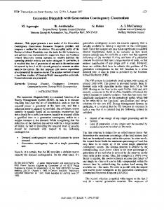
and an ellipsoid algorithm, for example, each having its own advantages and disadvantages. In this study, LINGO11, very mature software widely used in various mathematical optimization problems, is used to solve the quadratic programming algorithm problems. 3.3. Multiperiod Network Flow Model. A continuous time network flow is constituted by combining each network flow chart for a single period of time. A multiperiod model is a three-dimensional model with each layer corresponding to a single-period model (as shown in Figure 2). Each 𝑠𝑖 is united to form new 𝑠, and, in the same way, to form a new 𝑟. Arc(𝑠, 𝑠𝑖 ) represents the output and arc(𝑟𝑖 , 𝑟) represents the load. Considering each period together, a continuous-time power scheduling plan can be obtained. It is merely a schematic diagram, and the practical applications in power system may be more complex than that in Figure 2. For instance, the direction of the arcs in each layer may vary with different operating conditions. In order to simplify the analysis, we assume that the lines and transformers meet their capacity constraints. The above structure model (Figure 2) represents a typical generalized network flow programming problem. It can be expressed as min 𝐶𝑇 𝑋,
(19)
𝐴𝑋 = 𝑏,
(20)
satisfied with
where 𝐶 represents the 𝑚-dimensional arc cost vector; 𝑋 represents the 𝑚-dimensional arc flow; 𝑏 represents an 𝑛dimensional vector injected nodes; and 𝐴 represents 𝑛 × 𝑚 dimensional node-arc incidence matrix [39].
4. The Solution Process Diagram The steps in the procedure of ESGD (the low-carbon dispatching calculation process is the same) can be described as follows (as shown in Figure 3). Step 1. Determine the load 𝑃𝑡 at 𝑡 time according to the load forecasting curve, where 𝑇 represents the total of time periods. Step 2. Put 𝑃𝑡 as the flow at sink vertex.
Mathematical Problems in Engineering
5
Start
s
0
Load forecasting Pt (t = 1 : T)
4
6
1
5
2
3
7
r
Figure 5: Network diagram. ΣPload = Pt
Table 1: The parameters of transmission lines.
minΣFi (Pi ) s.t. constraints
No
t = T?
𝑉 (kV) 110 110 110 10 10
Line 𝐿1 𝐿2 𝐿3 𝐿4 𝐿5
t= t+1
𝑇 𝑇1 𝑇2
ESGD schedule
𝑉 (kV) 110/11 110/11
𝐿 (km) 71.2 71.2 71.2 10 10
𝑅 (Ω) 12.1 12.1 12.1 2.42 2.42
Model SFPL1-50000/110 SFPL1-50000/110
Δ𝑃𝑘 (kw) 250 250
𝑅𝑇 (Ω) 1.21 1.21
Table 3: The parameters of generators.
End
𝐺 𝐺1 𝐺2
Figure 3: Flowchart of solution procedure.
Capacity (MW) 100 100
Output limit 50 ≤ 𝑃𝐺1 ≤ 100 50 ≤ 𝑃𝐺2 ≤ 100
𝛼𝑖 0.0014 0.0018
𝛽𝑖 0.25 0.18
𝛾𝑖 2.5 5.0
PD3
PG1
1
4
L1
6 PD6
𝑟0 (Ω/km) 0.17 0.17 0.17 0.242 0.242
Table 2: The parameters of transformers.
Yes
L2
Model LGJ-185 LGJ-185 LGJ-185 LGJ-120 LGJ-120
L3
L5 T2
5 PD5
3
T1 L4
2 PG2
Figure 4: IEEE 6-bus power system diagram.
The corresponding cost flow network diagram is shown in Figure 5, in which the directed diagram of the system includes 8 vertexes and 12 arcs. In order to consider network losses, the net loss unit is turned into a standard coal consumption unit; that is, 1 MW = 0.123 t/h. In this model, the equivalent calorific value of 1 kg standard coal is 7000 kcal. The total-cost optimization model can be expressed as follows: min
Step 3. Solve the solution according to (1), satisfying the constraints (see (7) to (15)).
2 ) 𝐹 (𝑥) = (0.25𝑥01 + 0.0028𝑥01 2 ) + (0.18𝑥02 + 0.0036𝑥02
Step 4. If 𝑡 = 𝑇, then output ESGD scheduling results; otherwise, if 𝑡 < 𝑇, then let 𝑡 = 𝑡 + 1 and go to Step 2.
2 2 + 𝑥65 ) + 0.0002 × 0.123 × (𝑥43
5. Example Analysis
2 2 × (𝑥25 + 𝑥23 ) + 0.002 × 0.123
For this study, we calculated a modified IEEE 6-bus power system, which contains 2 generators, 2 transformers and 5 transmission lines (as shown in Figure 4). The parameters in the modified system are shown in Tables 1, 2, and 3. In the tables, 𝑟0 is the resistivity of a conductor per unit length, 𝐿 is the length of lines, 𝑅 and 𝑅𝑇 are the resistance of lines and transformers, respectively, Δ𝑃𝑘 represents short circuit loss of a transformer, and 𝛼𝑖 , 𝛽𝑖 , and 𝛾𝑖 refer to the cost coefficients of the 𝑖th generator (in Table 3).
2 2 2 + 𝑥46 + 𝑥16 ) × (𝑥14
+ 0.0004 × 0.123
s.t.
𝑥01 − 𝑥14 − 𝑥16 = 0 𝑥02 − 𝑥25 − 𝑥23 = 0 2 2 𝑥23 − 0.0002𝑥23 + 𝑥43 − 0.0001𝑥43 − 𝑥37 = 0 2 𝑥14 − 0.001𝑥14 − 𝑥46 − 𝑥43 = 0
6
Mathematical Problems in Engineering 2 2 𝑥65 − 0.0001𝑥65 + 𝑥25 − 0.0002𝑥25 − 𝑥57 = 0
+ 𝑥16 −
2 0.001𝑥16
− 𝑥65 − 𝑥67 = 0
𝑥37 + 𝑥57 + 𝑥67 = 𝑃𝐷3 + 𝑃𝐷5 + 𝑃𝐷6 50 ≤ 𝑥01 ≤ 100,
100
s 0 200
0 ≤ 𝑥14 ≤ 100,
0 ≤ 𝑥46 ≤ 100,
0 ≤ 𝑥16 ≤ 100,
0 ≤ 𝑥43 ≤ 50,
0 ≤ 𝑥25 ≤ 100,
0 ≤ 𝑥65 ≤ 50,
0 ≤ 𝑥23 ≤ 100,
0 ≤ 𝑥67 ≤ 100,
0 ≤ 𝑥57 ≤ 100,
0 ≤ 𝑥37 ≤ 100,
48.1
53.3
41.6
1
5
50
100
50 ≤ 𝑥02 ≤ 100,
6
51.9
2
3
50
49.5
7
r 193.8
91
Figure 6: The minimal cost flow under maximum flow. 2.1
4 s 100
50
0
(21)
21.3
1
5
25 2
25
3
27.5 24.9
7
r 98.5
46.1
Figure 7: The minimal cost flow distribution under minimum flow.
P (MW)
where 𝑥 refers to the flow in the network; then the objective function is obviously a convex cost flow problem and a quadratic programming method can be used to solve it. When the load changes, as shown in Figure 8, the differing distribution of the minimum cost flow can be concluded and, therefore, a continuous dispatch result can be obtained. In order to simplify the analysis, we assumed that all units run within a safe operation area. The ramp rate limit of 100 MW unit is 2 MW/min, so the ramp rate limits can meet the requirements created when the time interval is an hour. We also assumed that the reactive power can be compensated locally and the system does not transmit reactive power. The voltage of nodes was kept within their specified ratings, and the reserve capacity of the grid was assumed to meet operational requirements. Additionally, the test was performed on an Intel (R) Pentium (R) CPU 2.13 GHz 2.0 GB RAM with LINGO11, and the average iteration times were 58. The maximum flow that can pass the network and the corresponding minimal cost distribution is shown in Figure 6. The minimum flow distribution of the minimum cost flow is shown in Figure 7. The load and corresponding minimal coal consumption are listed in Table 4 and shown in Figure 8, respectively. Where 𝑇 is the time period (h), 𝑃 is the power of load (MW) and 𝐹 is the coal consumption (t/h). Electricity and minimal coal consumption accumulation are listed in Table 5 and shown in Figure 10, respectively. 𝑆 refers to the accumulation of coal consumption (t) and 𝑊 refers to accumulation of electricity (MWh). It can be seen that the accumulated electricity will gradually increase with the increase of time. The same trend occurs with the accumulated minimal coal consumption. Unit scheduling results are shown in Figure 9. According to the electrical-carbon conversion relations, 2.77 tons of CO2 can be emitted for 1 ton of standard coal consumed. In addition, the minimum CO2 emissions and the accumulation curve can also be obtained (as shown in Figures 11 and 12). The value of CO2 emissions and its accumulation are listed in Table 6, where 𝐶𝑒 and 𝐶𝑎 refer to CO2 emissions and its accumulation value, respectively.
50
6
26
24
200
120
180
100
160
80
140
60
120
40
100
0
5
10
15
20
F (t/h)
𝑥46 −
2 0.001𝑥46
4.2
4
20 25
T (h) F P
Figure 8: Load and coal consumption curve.
We can see that the emissions of CO2 change with the power load by the same regularity, which reflects that the objectives of low-carbon generation dispatching and energysaving generation dispatching are consistent. In order to support our findings, we also solved this same problem by invoking the CPLEX solver in the MATLAB toolbox YALMIP [40]. The extended solver of LINGO11 includes Branch-and-Bound solver, Global solver, and Multistart solver, while the solver in CPLEX is mainly based on interior-point method. If these two different methods come to a same conclusion, then the result concluded is credible. The result by CPLEX produced the same solution garnered using LINGO11, which proves the correctness of the method used in this study.
6. Conclusions The minimal cost flow algorithm can be used to dispatch the power system and can reflect the system network topology, making it fairly easy to consider system constraints.
Mathematical Problems in Engineering
7 Table 4: Load and coal consumption.
𝑇 (h) 𝑃 (MW) 𝐹 (t/h) 𝑇 (h) 𝑃 (MW) 𝐹 (t/h)
1 110 44.58 13 130 57.39
2 100 38.74 14 140 64.36
3 110 44.58 15 150 71.71
4 120 50.80 16 160 79.45
5 130 57.39 17 170 87.58
6 140 64.36 18 180 96.10
7 150 71.71 19 190 105.0
8 160 79.45 20 180 96.10
9 170 87.58 21 170 87.58
10 160 79.45 22 150 71.71
11 150 71.71 23 130 57.39
12 140 64.36 24 120 50.80
9 539.2 1190 21 1500 3110
10 618.6 1350 22 1571 3260
11 690.4 1500 23 1629 3390
12 754.7 1640 24 1680 3510
10 220.1 1714 22 198.6 4353
11 198.6 1912 23 159.0 4513
12 178.3 2091 24 140.7 4653
Table 5: Electricity and coal consumption accumulation. 𝑇 (h) 𝑆 (t) 𝑊 (MWh) 𝑇 (h) 𝑆 (t) 𝑊 (MWh)
1 44.6 110 13 812.1 1770
2 83.3 210 14 876.5 1910
3 127.9 320 15 948.2 2060
4 178.7 440 16 1027 2220
5 236.1 570 17 1115 2390
6 300.5 710 18 1211 2570
7 372.2 860 19 1316 2760
8 451.6 1020 20 1412 2940
𝑇 (h) 𝐶𝑒 (t) 𝐶𝑎 (t) 𝑇 (h) 𝐶𝑒 (t) 𝐶𝑎 (t)
1 123.5 123.5 13 159.0 2249
2 107.3 230.8 14 178.3 2428
3 123.5 354.3 15 198.6 2626
4 140.7 495.0 16 220.1 2846
5 159.0 654.0 17 242.6 3089
6 178.3 832.3 18 266.2 3355
7 198.6 1031 19 290.9 3646
80
W (MWh)
P (MW)
100
60 40
5
0
10
15
20
8 220.1 1251 20 266.2 3912
9 242.6 1494 21 242.6 4155
4000
4000
3000
3000
2000
2000
1000
1000
0
25
T (h)
0
5
10
15
S(t)
Table 6: The value of CO2 emissions and CO2 emissions accumulation.
0 25
20
T (h)
G1 G2
S W
Figure 9: Outputs of generators.
Figure 10: Electricity and coal consumption accumulation curve. 300 250 CO2 (t)
The method is simple, rapid, and clear in terms basic concepts. The example analysis proves that the method is feasible and practical. In order to simplify the analysis, this study only considers the energy-saving scheduling of thermal units, without considering the effects of hydropower, wind power, and other renewable energy sources: although they do not consume coal and discharge CO2 , they do have an impact on load-flow distribution and network losses in power systems. Accordingly, the next step will be to initiate research to study the influences of renewable energy sources on ESGD in power systems.
200 150 100
0
5
10
15 T (h)
Figure 11: CO2 emissions curve.
20
25
8
Mathematical Problems in Engineering
CO2 (t)
6000
[11]
4000 2000
[12] 0
0
5
10
15
20
25
T (h)
Figure 12: CO2 emissions accumulation curve.
Conflict of Interests The authors declare that there is no conflict of interests regarding the publication of this paper.
[13]
[14]
[15]
Acknowledgments The authors would like to acknowledge the guidance and support from their colleagues and supervisor, along with great thanks to Prof. Galen Leonhardy for editorial assistance.
References [1] W. Yu and B. G. Xin, “Governance mechanism for global greenhouse gas emissions: a stochastic differential game approach,” Mathematical Problems in Engineering, vol. 2013, Article ID 312585, 13 pages, 2013. [2] H. M. Ndiritu, K. Kibicho, and B. B. Gathitu, “Influence of flow parameters on capture of carbon dioxide gas by a wet scrubber,” Journal of Power Technologies, vol. 93, no. 1, pp. 9–15, 2013. [3] Y.-C. Chang, T.-S. Chan, and W.-S. Lee, “Economic dispatch of chiller plant by gradient method for saving energy,” Applied Energy, vol. 87, no. 4, pp. 1096–1101, 2010. [4] J. Kotowicz and P. Lukowicz, “Influence of chosen parameters on economic effectiveness of a supercritical combined heat and power plant,” Journal of Power Technologies, vol. 93, no. 5, pp. 323–329, 2013. [5] C.-T. Cheng, S.-S. Li, and G. Li, “A hybrid method of incorporating extended priority list into equal incremental principle for energy-saving generation dispatch of thermal power systems,” Energy, vol. 64, no. 1, pp. 688–696, 2014. [6] G.-C. Liao, “A novel evolutionary algorithm for dynamic economic dispatch with energy saving and emission reduction in power system integrated wind power,” Energy, vol. 36, no. 2, pp. 1018–1029, 2011. [7] R. A. Jabr, A. H. Coonick, and B. J. Cory, “A homogeneous linear programming algorithm for the security constrained economic dispatch problem,” IEEE Transactions on Power Systems, vol. 15, no. 3, pp. 930–936, 2000. [8] R. A. Jabr, A. H. Coonick, and B. J. Cory, “A primal-dual interior point method for optimal power flow dispatching,” IEEE Transactions on Power Systems, vol. 17, no. 3, pp. 654–662, 2002. [9] W. Ongsakul and N. Petcharaks, “Unit commitment by enhanced adaptive Lagrangian relaxation,” IEEE Transactions on Power Systems, vol. 19, no. 1, pp. 620–628, 2004. [10] H. Zhong, Q. Xia, Y. Wang, and C. Kang, “Dynamic economic dispatch considering transmission losses using quadratically
[16]
[17]
[18]
[19]
[20]
[21]
[22]
[23]
[24]
[25]
constrained quadratic program method,” IEEE Transactions on Power Systems, vol. 28, no. 3, pp. 2232–2241, 2013. N. Sinsuphan, U. Leeton, and T. Kulworawanichpong, “Optimal power flow solution using improved harmony search method,” Applied Soft Computing Journal, vol. 13, no. 5, pp. 2364–2374, 2013. J. J. Hargreaves and B. F. Hobbs, “Commitment and dispatch with uncertain wind generation by dynamic programming,” IEEE Transactions on Sustainable Energy, vol. 3, no. 4, pp. 724– 734, 2012. J. Soares, M. Silva, T. Sousa, Z. Vale, and H. Morais, “Distributed energy resource short-term scheduling using Signaled Particle Swarm Optimization,” Energy, vol. 42, no. 1, pp. 466–476, 2012. ¨ on, “Solution to scalarized environmental C. Yas¸ar and S. Ozy¨ economic power dispatch problem by using genetic algorithm,” International Journal of Electrical Power and Energy Systems, vol. 38, no. 1, pp. 54–62, 2012. M. H. Gomes and J. T. Saraiva, “A market based active/reactive dispatch including transformer taps and reactor and capacitor banks using simulated Annealing,” Electric Power Systems Research, vol. 79, no. 6, pp. 959–972, 2009. P. Somasundaram and K. Kuppusamy, “Application of evolutionary programming to security constrained economic dispatch,” International Journal of Electrical Power and Energy Systems, vol. 27, no. 5-6, pp. 343–351, 2005. S. Pothiya, I. Ngamroo, and W. Kongprawechnon, “Ant colony optimisation for economic dispatch problem with non-smooth cost functions,” International Journal of Electrical Power and Energy Systems, vol. 32, no. 5, pp. 478–487, 2010. M. Sharma, M. Pandit, and L. Srivastava, “Reserve constrained multi-area economic dispatch employing differential evolution with time-varying mutation,” International Journal of Electrical Power and Energy Systems, vol. 33, no. 3, pp. 753–766, 2011. J. S. Alsumait, J. K. Sykulski, and A. K. Al-Othman, “A hybrid GA-PS-SQP method to solve power system valve-point economic dispatch problems,” Applied Energy, vol. 87, no. 5, pp. 1773–1781, 2010. J. Cai, Q. Li, L. Li, H. Peng, and Y. Yang, “A hybrid CPSO-SQP method for economic dispatch considering the valve-point effects,” Energy Conversion and Management, vol. 53, no. 1, pp. 175–181, 2012. C. C. A. Rajan, “A solution to the economic dispatch using EP based SA algorithm on large scale power system,” International Journal of Electrical Power & Energy Systems, vol. 32, no. 6, pp. 583–591, 2010. M. Basu, “Hybridization of bee colony optimization and sequential quadratic programming for dynamic economic dispatch,” International Journal of Electrical Power and Energy Systems, vol. 44, no. 1, pp. 591–596, 2013. A. R. L. Oliveira, S. Soares, and L. Nepomuceno, “Optimal active power dispatch combining network flow and interior point approaches,” IEEE Transactions on Power Systems, vol. 18, no. 4, pp. 1235–1240, 2003. J. Zhu and J. A. Momoh, “Multi-area power systems economic dispatch using nonlinear convex network flow programming,” Electric Power Systems Research, vol. 59, no. 1, pp. 13–20, 2001. C. Li, Y. Liu, Y. Cao, Y. Tan, C. Xue, and S. Tang, “Consistency evaluation of low-carbon generation dispatching and energysaving generation dispatching,” Proceedings of the Chinese Society of Electrical Engineering, vol. 31, no. 31, pp. 94–101, 2011.
Mathematical Problems in Engineering [26] S. S. Reddy, B. K. Panigrahi, R. Kundu, R. Mukherjee, and S. Debchoudhury, “Energy and spinning reserve scheduling for a wind-thermal power system using CMA-ES with mean learning technique,” International Journal of Electrical Power and Energy Systems, vol. 53, no. 1, pp. 113–122, 2013. [27] C.-C. Kuo, “Generation dispatch under large penetration of wind energy considering emission and economy,” Energy Conversion and Management, vol. 51, no. 1, pp. 89–97, 2010. [28] A. Immanuel Selvakumar, “Enhanced cross-entropy method for dynamic economic dispatch with valve-point effects,” International Journal of Electrical Power and Energy Systems, vol. 33, no. 3, pp. 783–790, 2011. [29] R. Azizipanah-Abarghooee, T. Niknam, A. Roosta, A. R. Malekpour, and M. Zare, “Probabilistic multiobjective windthermal economic emission dispatch based on point estimated method,” Energy, vol. 37, no. 1, pp. 322–335, 2012. [30] M. A. Abido, “Multiobjective particle swarm optimization for environmental/economic dispatch problem,” Electric Power Systems Research, vol. 79, no. 7, pp. 1105–1113, 2009. [31] F.-R. Xie and R.-A. Jia, “Nonlinear fixed charge transportation problem by minimum cost flow-based genetic algorithm,” Computers & Industrial Engineering, vol. 63, no. 4, pp. 763–778, 2012. [32] G. T. Heineman, G. Pollice, and S. Selkow, Algorithms in a Nutshell, O’Reilly Media, Sebastopol, Calif, USA, 2008. [33] F. S. Hillier and G. J. Lieberman, Introduction to Operations Research, McGraw-Hill, 9th edition, 2010. [34] R. K. Ahuja, T. L. Magnanti, and J. Orlin, Network Flows: Theory, Algorithms and Applications, Prentice Hall, Englewood Cliffs, NJ, USA, 1993. [35] F. Curtis and J. Nocedal, “Steplength selection in interior-point methods for quadratic programming,” Applied Mathematics Letters, vol. 20, no. 5, pp. 516–523, 2007. [36] M. D’ Apuzzo and M. Marino, “Parallel computational issues of an interior point method for solving large bound-constrained quadratic programming problems,” Parallel Computing: Theory and Applications, vol. 29, no. 4, pp. 467–483, 2003. [37] W. Cheng, Z. Chen, and D.-H. Li, “An active set truncated Newton method for large-scale bound constrained optimization,” Computers & Mathematics with Applications, vol. 67, no. 5, pp. 1016–1023, 2014. [38] M.-T. Yu, T.-Y. Lin, and C. Hung, “Active-set sequential quadratic programming method with compact neighbourhood algorithm for the multi-polygon mass production cutting-stock problem with rotatable polygons,” International Journal of Production Economics, vol. 121, no. 1, pp. 148–161, 2009. [39] Z.-A. Zhang and X.-G. Cai, “Power purchase plan using minimal cost flow,” Computer Modelling and New Technologies, vol. 18, no. 2, pp. 281–285, 2014. [40] J. L¨ofberg, “YALMIP: a toolbox for modeling and optimization in MATLAB,” in Proceedings of the IEEE International Symposium on Computer Aided Control System Design, pp. 284–289, Taipei, Taiwan, September 2004.
9
Advances in
Operations Research Hindawi Publishing Corporation http://www.hindawi.com
Volume 2014
Advances in
Decision Sciences Hindawi Publishing Corporation http://www.hindawi.com
Volume 2014
Journal of
Applied Mathematics
Algebra
Hindawi Publishing Corporation http://www.hindawi.com
Hindawi Publishing Corporation http://www.hindawi.com
Volume 2014
Journal of
Probability and Statistics Volume 2014
The Scientific World Journal Hindawi Publishing Corporation http://www.hindawi.com
Hindawi Publishing Corporation http://www.hindawi.com
Volume 2014
International Journal of
Differential Equations Hindawi Publishing Corporation http://www.hindawi.com
Volume 2014
Volume 2014
Submit your manuscripts at http://www.hindawi.com International Journal of
Advances in
Combinatorics Hindawi Publishing Corporation http://www.hindawi.com
Mathematical Physics Hindawi Publishing Corporation http://www.hindawi.com
Volume 2014
Journal of
Complex Analysis Hindawi Publishing Corporation http://www.hindawi.com
Volume 2014
International Journal of Mathematics and Mathematical Sciences
Mathematical Problems in Engineering
Journal of
Mathematics Hindawi Publishing Corporation http://www.hindawi.com
Volume 2014
Hindawi Publishing Corporation http://www.hindawi.com
Volume 2014
Volume 2014
Hindawi Publishing Corporation http://www.hindawi.com
Volume 2014
Discrete Mathematics
Journal of
Volume 2014
Hindawi Publishing Corporation http://www.hindawi.com
Discrete Dynamics in Nature and Society
Journal of
Function Spaces Hindawi Publishing Corporation http://www.hindawi.com
Abstract and Applied Analysis
Volume 2014
Hindawi Publishing Corporation http://www.hindawi.com
Volume 2014
Hindawi Publishing Corporation http://www.hindawi.com
Volume 2014
International Journal of
Journal of
Stochastic Analysis
Optimization
Hindawi Publishing Corporation http://www.hindawi.com
Hindawi Publishing Corporation http://www.hindawi.com
Volume 2014
Volume 2014