Enhancing Collaborative Filtering by User-User Covariance Matrix

Hindawi Mathematical Problems in Engineering Volume 2018, Article ID 9740402, 9 pages https://doi.org/10.1155/2018/9740402

Research Article Enhancing Collaborative Filtering by User-User Covariance Matrix Yingyuan Xiao ,1,2 Jingjing Shi,1,2 Wenguang Zheng,1,2 Hongya Wang,3 and Ching-Hsien Hsu 4 1

Key Laboratory of Computer Vision and System, Ministry of Education, 300384 Tianjin, China Tianjin Key Laboratory of Intelligence Computing and Novel Software Technology, China 3 Donghua University, 201620 Shanghai, China 4 Chung Hua University, 30012 Hsinchu, Taiwan 2

Correspondence should be addressed to Yingyuan Xiao; xiaoyingyuan [email protected] Received 11 August 2018; Revised 10 October 2018; Accepted 4 November 2018; Published 25 November 2018 Academic Editor: Emilio Insfran Pelozo Copyright © 2018 Yingyuan Xiao et al. This is an open access article distributed under the Creative Commons Attribution License, which permits unrestricted use, distribution, and reproduction in any medium, provided the original work is properly cited. The collaborative filtering (CF) approach is one of the most successful personalized recommendation methods so far, which is employed by the majority of personalized recommender systems to predict users’ preferences or interests. The basic idea of CF is that if users had the same interests in the past they will also have similar tastes in the future. In general, the traditional CF may suffer the following problems: (1) The recommendation quality of CF based system is greatly affected by the sparsity of data. (2) The traditional CF is relatively difficult to adapt the situation that users’ preferences always change over time. (3) CF based approaches are used to recommend similar items to a user ignoring the user’s demand for variety. In this paper, to solve the above problems we build a new user-user covariance matrix to replace the traditional CF’s user-user similarity matrix. Compared with the user-user similarity matrix, the user-user covariance matrix introduces the user-user covariance to finely describe the changing trends of users’ interests. Furthermore, we propose an enhancing collaborative filtering method based on the user-user covariance matrix. The experimental results show that the proposed method can significantly improve the diversity of recommendation results and ensure the good recommendation precision.

1. Introduction Recommendation systems have been widely applied to deal with information overload problems in e-commerce sites [1]. It is well known that collaborative filtering (CF) is one of the most widely used methods in recommender systems. CF utilizes users’ behaviors (e.g., ratings or clicks) to infer a target user’s preference for a particular item. CF is based on the assumption that users’ previous behaviors have huge influence on their future behaviors. The basic idea of CF is that if users shared the same interests in the past they will also have similar tastes in the future. Although CF approach has been employed by the majority of traditional personalized recommender systems, CF approach usually faces the following challenges: (1) The sparse data of the user-item matrix seriously affect the recommendation quality. (2) The traditional CF is relatively difficult to adapt

the situation that users’ preferences always change over time. (3) Always recommending similar items to a user will fail to meet the user’s demand for variety. In this paper, we propose an enhancing collaborative f iltering method based on covariance matrix named CFCM, such that the problems described above can be solved. We first construct the user-user covariance matrix according to the traditional user-item rating matrix, which alleviates the sparsity of the rating matrix. Secondly, we introduce the covariance to effectively capture the user’s interest change. Finally, we adjust the weight between positive and negative reverse recommendations to improve the diversity of CF methods. The experimental results on a large MovieLens dataset demonstrate that CFCM outperforms the state-ofthe-art CF methods. The rest of this paper is organized as follows. Section 2 reviews related work. Section 3 builds a new user-user

2

Mathematical Problems in Engineering

covariance matrix and presents an enhancing collaborative filtering method. Section 4 evaluates the proposed method through extensive experiments, and Section 5 concludes this paper.

CF approach is one of the most successful personalized recommendation methods. The CF approach was first proposed by Goldberg et al. [2]. Since then, many improved CF methods have been proposed for personalized recommendation. CF methods can be grouped into two categories: memorybased and model-based. The model-based CF approaches leverage training datasets to train a predefined model [3–8]. The memorybased CF approaches are most relevant to the method proposed in this paper. At present, the memory-based CF approaches are widely adopted in commercial personalized recommender systems [9, 10]. The key to these memorybased CF approaches is how to efficiently compute the similarity between two users. Then, for a particular user, his neighborhood can be determined according to the similarity and recommendations are made based on the rating of neighborhood of the target user. Many similarity measures (i.e., similarity functions) for these memory-based CF approaches have been proposed. In the following, we use 𝑈 to denote the set of users, I to represent the set of items, 𝐼𝑢 to denote the set of those items rated by user u, and 𝑅 to denote the user-item rating matrix. The user-item rating matrix 𝑅 is a |𝑈| × |𝐼| matrix, and each entry 𝑟𝑢𝑖 of 𝑅 represents the 󳨀 rating of user 𝑢 for item 𝑖. Let → 𝑟𝑢 denote the rating vector → 󳨀 of user u; i.e., 𝑟𝑢 is a |𝐼|-dimensional vector constructed by all entries 𝑟𝑢𝑖 , where 𝑖 ∈ 𝐼. We use 𝑟𝑢 to denote the average rating value of user 𝑢 and 𝑟𝑚𝑒𝑑 to denote the median value of all rates in the user-item rating matrix R. Given two users 𝑢 and V, a similarity function 𝑠𝑖𝑚(𝑢, V) returns a value that indicates the similarity of the two users. The larger the value is, the more similar the two users are. The cosine similarity is one of the widely used similarity functions. The cosine similarity function is defined as follows:

(1)

The Pearson correlation coefficient (PCC) [11] is another of the most popular similarity measures for CF approaches. The PCC similarity function is defined by the following equation: 𝑠𝑖𝑚𝑝𝑐𝑐 (𝑢, V) =

∑𝑖∈𝐼𝑢 ∩𝐼V (𝑟𝑢𝑖 − 𝑟𝑢 ) × (𝑟V𝑖 − 𝑟V )

𝑠𝑖𝑚𝑐𝑝𝑐𝑐 (𝑢, V) =

2. Related Work

→ → 󳨀 ∑𝑖∈𝐼 𝑟𝑢𝑖 × 𝑟V𝑖 .𝑟 𝑟𝑢 󳨀 V 𝑠𝑖𝑚𝑐𝑜𝑠 (𝑢, V) = 󵄩󵄩→ 󵄩 󵄩󵄩→ 󵄩󵄩 = 󳨀 󵄩 2 2 󵄩󵄩󳨀 󵄩 󵄩 󵄩 󵄩𝑟𝑢 󵄩󵄩 × 󵄩󵄩 𝑟V 󵄩󵄩 √∑𝑖∈𝐼 𝑟𝑢𝑖 × √∑𝑖∈𝐼 𝑟V𝑖

to replace the mean value of the specified user’ ratings used in PCC. The CPCC similarity function is formulated as follows:

(2)

√∑𝑖∈𝐼 ∩𝐼 (𝑟𝑢𝑖 − 𝑟𝑢 )2 × √∑𝑖∈𝐼 ∩𝐼 (𝑟V𝑖 − 𝑟V )2 𝑢 V 𝑢 V

A variant of PCC is the constrained Pearson correlation coefficient (CPCC) [12]. The difference between CPCC and PCC is that CPCC uses the median value of all users’ ratings

∑𝑖∈𝐼𝑢 ∩𝐼V (𝑟𝑢𝑖 − 𝑟𝑚𝑒𝑑 ) × (𝑟V𝑖 − 𝑟𝑚𝑒𝑑 )

(3)

√∑𝑖∈𝐼 ∩𝐼 (𝑟𝑢𝑖 − 𝑟𝑚𝑒𝑑 )2 × √∑𝑖∈𝐼 ∩𝐼 (𝑟V𝑖 − 𝑟𝑚𝑒𝑑 )2 𝑢 V 𝑢 V

Jaccard and mean squared difference (MSD) are also commonly used as similarity measures [13]. Their similarity functions are, respectively, defined as follows: 󵄨󵄨 󵄨 󵄨𝐼 ∩ 𝐼 󵄨󵄨 𝑠𝑖𝑚𝐽𝑎𝑐 (𝑢, V) = 󵄨󵄨󵄨 𝑢 V 󵄨󵄨󵄨 󵄨󵄨𝐼𝑢 ∪ 𝐼V 󵄨󵄨 (4) 2 ∑𝑖𝜖𝐼 (𝑟𝑢𝑖 − 𝑟V𝑖 ) 𝑠𝑖𝑚𝑀𝑆𝐷 (𝑢, V) = 1 − 󵄨󵄨 󵄨 󵄨󵄨𝐼𝑢 ∪ 𝐼V 󵄨󵄨󵄨 Further, Bobadilla et al. [14] combine Jaccard and MSD and propose a new similarity measure called JMSD. JMSD is defined as the following equation: 𝑠𝑖𝑚𝐽𝑀𝑆𝐷 (𝑢, V) = 𝑠𝑖𝑚𝐽𝑎𝑐 (𝑢, V) × 𝑠𝑖𝑚𝑀𝑆𝐷 (𝑢, V)

(5)

In addition, more works on similarity measures [15–19] have been investigated. Bobadilla et al. [15] present a new similarity measure, called MJD, which leverages optimization based on neural learning to combine the existing similarity measures. Ahn [16] proposes a new heuristic similarity measure called PIP (Proximity-Impact-Popularity), which is composed of three factors (proximity, impact, and popularity) of similarity and utilizes domain specific interpretation of user ratings to overcome the cold-start problem. Pirasteh et al. [17] introduce new weighting schemes and propose a new similarity measure called AC-PCC. AC-PCC allows us to consider new features in finding similarities between users. Liu et al. [18] present a new user similarity model (NHSM) to improve the recommendation performance when only few ratings are available to calculate the similarities. NHSM considers the local context information of user ratings to infer a target user’s preference for a particular item. Patraet al. [19] propose BCF similarity measure, which utilizes all ratings information comprehensively for locating useful neighbors of an active user in sparse ratings dataset. Obviously, the existing traditional similarity measures focus on how to infer a target user’s local preference based on his/her similar users’ previous behaviors and ignore more or less the fact that a user’s preference or interest always changes dynamically. In addition, ensuring the diversity of recommendations is often a desirable feature in recommender systems. Therefore, how to truly reflect the change of user’s interest is an important issue in designing a similarity function. In this paper, we introduce a novel method by using covariance to depict the changing trends of users’ interests and build a new user-user covariance matrix to model user similarity.

3. Enhancing Collaborative Filtering Approach In this section, we first introduce covariance to build a new user-user covariance matrix and then propose an enhancing

Mathematical Problems in Engineering

3 Table 1: A user-user covariance matrix.

collaborative filtering method based on the user-user covariance matrix. 3.1. User-User Covariance Matrix. In probability theory and statistics, covariance is a measure of the joint variability of two random variables. If the trend of the two variables is consistent, the covariance between the two variables is positive. In the opposite case, if two variables change in the opposite direction, the covariance between the two variables is negative. The sign of the covariance therefore shows the tendency in the linear relationship between the variables. Considering the above-mentioned statistical characteristics of covariance, we construct a new user-user covariance matrix to model user similarity. Let 𝑢𝑖 and 𝑢𝑗 denote any two users in U, |𝑈| =m, I represent the set of items, 𝐼𝑖 represent the set of items rated by 𝑢𝑖 , 𝐼𝑗 denote the set of items rated by 𝑢𝑗 , rik denote the rating of user 𝑢𝑖 for item 𝑖𝑘 , and rjk represent the rating of user 𝑢𝑗 for item 𝑖𝑘 . Now, we formally define the user-user covariance matrix. Definition 1. A user-user covariance matrix is an 𝑚 × 𝑚 matrix, denoted by 𝐶 = {𝑐𝑖𝑗 }𝑚×𝑚 , where 𝑐𝑖𝑗 = 𝑐𝑜V (𝑢𝑖 , 𝑢𝑗 ) {+∞, ={ 𝐸 [(𝑢𝑖 − 𝐸 (𝑢𝑖 )) . (𝑢𝑗 − 𝐸 (𝑢𝑗 ))] , {

𝑖=𝑗

(6)

𝑖 ≠ 𝑗

In the above definition, cov(𝑢𝑖 , 𝑢𝑗 ) is set to +∞, when i = j. When 𝑖 ≠ 𝑗, cov(𝑢𝑖 , 𝑢𝑗) denotes the covariance between 𝑢𝑖 and 𝑢𝑗 . Since each user is modeled as the rating sequence for all items in CF approaches, we can consider a user as a random variable, which means that it makes sense to calculate the covariance between two users. Like the covariance between two variables in probability theory and statistics, we give the calculation method for the covariance between two users at 𝑖 ≠ 𝑗 in 𝑐𝑜V (𝑢𝑖 , 𝑢𝑗 ) = 𝐸 [(𝑢𝑖 − 𝐸 (𝑢𝑖 )) ∙ (𝑢𝑗 − 𝐸 (𝑢𝑗 ))] = 𝐸 (𝑢𝑖 𝑢𝑗 ) − 𝐸 (𝑢𝑖 ) 𝐸 (𝑢𝑗 ) =

1 1 ∑𝑟𝑖𝑘 .𝑟𝑗𝑘 − 2 ∑𝑟𝑖𝑘 .∑𝑟𝑗𝑘 |𝐼| 𝑘∈𝐼 |𝐼| 𝑘∈𝐼 𝑘∈𝐼

=

1 1 ∑ 𝑟 .𝑟 − ∑ 𝑟 .∑𝑟 |𝐼| 𝑘∈(𝐼 ∩𝐼 ) 𝑖𝑘 𝑗𝑘 |𝐼|2 𝑘∈𝐼 𝑖𝑘 𝑘∈𝐼 𝑗𝑘 𝑖 𝑗

(7)

Below we use an example to illustrate how to use (7) 󳨀 to calculate the covariance between two users. let → 𝑟1 = (𝑟11 , 𝑟12 , 𝑟13 , 𝑟14 , 𝑟15 , 𝑟16 ) = (0, 5, 2, 0, 3, 0) denote the rating 󳨀 𝑟2 = vector of user 𝑢1 for items 𝑖1 , 𝑖2 , 𝑖3 , 𝑖4 , 𝑖5 , and 𝑖6 , and → (𝑟21 , 𝑟22 , 𝑟23 , 𝑟24 , 𝑟25 , 𝑟26 ) = (4, 0, 0, 3, 0, 4) represent the rating vector of user 𝑢2 for items 𝑖1 , 𝑖2 , 𝑖3 , 𝑖4 , 𝑖5 , and 𝑖6 . According to (7), the covariance cov(𝑢1 , 𝑢2 ) between 𝑢1 and 𝑢2 is calculated as follows: 𝑐𝑜V(𝑢1 , 𝑢2 ) = (1/|𝐼|) ∑𝑘∈(𝐼1 ∩𝐼2 ) 𝑟1𝑘 .𝑟2𝑘 − (1/|𝐼|2 ) ∑𝑘∈𝐼 𝑟1𝑘 . ∑𝑘∈𝐼 𝑟2𝑘 , where 𝐼1 = {𝑖2 , 𝑖3 , 𝑖5 }, 𝐼2 = {𝑖1 , 𝑖4 , 𝑖6 }, 𝐼 = {𝑖1 , 𝑖2 ,

𝑢1 𝑢2 𝑢3 𝑢4 𝑢5

𝑢1 +∞ -3.056 -0.444 -2.222 2.222

𝑢2 -3.056 +∞ 0.111 2.389 -1.972

𝑢3 -0.444 0.111 +∞ -0.889 1.222

𝑢4 -2.222 2.389 -0.889 +∞ -2.889

𝑢5 2.222 -1.972 1.222 -2.889 +∞

Table 2: A user-item rating matrix. 𝑢1 𝑢2 𝑢3 𝑢4 𝑢5

𝑖1 null 4 null 5 null

𝑖2 5 null null null 5

𝑖3 2 null 2 null 5

𝑖4 null 3 null 3 null

𝑖5 3 null null null null

𝑖6 null 4 2 null 3

𝑖3 , 𝑖4 , 𝑖5 , 𝑖6 }, 𝐼1 ∩ 𝐼2 = {𝑖2 , 𝑖3 , 𝑖5 } ∩ {𝑖1 , 𝑖4 , 𝑖6 } = 0, and |𝐼| = 6. That is, cov(𝑢1 , 𝑢2 ) = 1/6 × 0 − (1/62 )(𝑟11 + 𝑟12 + 𝑟13 + 𝑟14 +𝑟15 + 𝑟16 ) × (𝑟21 + 𝑟22 + 𝑟23 + 𝑟24 +𝑟25 + 𝑟26 ) = 0 − (1/36)(0 + 5 + 2 + 0 + 3 + 0) × (4 + 0 + 0 + 3 + 0 + 4) ≈ −3.056. Further, Table 1 demonstrates a user-user covariance matrix, which is derived by (7) from a user-item rating matrix shown in Table 2. As shown in Table 1, a useruser covariance matrix is a symmetric matrix and adds the negative correlation to depict the opposite trends of users’ interests. For traditional similarity measures, if two users have no common rated items, the similarity between the two users is usually equal to zero. For example, the similarity between 𝑢1 and 𝑢2 is equal to the similarity between 𝑢1 and 𝑢4 , and both values are zero according to the traditional similarity measures, because 𝑢1 have no common rated items with 𝑢2 and 𝑢4 , as shown in Table 2. This means that the traditional similarity measures cannot distinguish the degree of dissimilarity between the users who have no common rated items. However, we can find from Table 1 that the covariance cov(𝑢1 , 𝑢2 ) between 𝑢1 and 𝑢2 is different from the covariance cov(𝑢1 , 𝑢4 ) between 𝑢1 and 𝑢4 , both values are negative, and the absolute value of cov(𝑢1 , 𝑢2 ) is bigger than that of cov(𝑢1 , 𝑢4 ). It means that 𝑢2 is more disinterested in those items, which 𝑢1 are of interest to, than 𝑢4 . From the above example, we can learn that the user-user covariance matrix has a finer description capability for user similarity trends, and especially for the users without common rated items, it shows the more powerful description capability than the traditional similarity measures. 3.2. The Proposed Collaborative Filtering Algorithm. In the proposed enhancing collaborative f iltering method based on covariance matrix (CFCM), we first build the user-user covariance matrix 𝐶 = {𝑐𝑖𝑗 }𝑚×𝑚 based on the user-item rating matrix. The above Definition 1 and (7) give the way of computing 𝐶 = {𝑐𝑖𝑗 }𝑚×𝑚 . Then, for any target user u, we employ the user-user covariance matrix to calculate its 𝐾 neighbors with the most similar interested trends and opposite 𝐾 neighbors with the most dissimilar interested

4

Mathematical Problems in Engineering Table 3: The basic attributes of MovieLens-1M.

Dataset MovieLens-1M

Number of users

Number of Movies

Number of Ratings

Sparsity level

Rating domain

6040

3706

1M

4.2%

{1, 2, 3, 4, 5}

Input: 𝑅 and 𝑢, where 𝑅 is the user-item rating matrix and 𝑢 denotes a target user. Output: Result, i.e., the recommendation list for 𝑢. 1: Result fl ⌀; 𝑁𝑢,𝑠 fl ⌀; 𝑁𝑢,𝑑 fl ⌀; Orderlistfl ⌀; 2: build the user-user covariance matrix 𝐶 = {𝑐𝑖𝑗 }𝑚×𝑚 based on 𝑅; 3: 𝑁𝑢,𝑠 fl GetKSimilarUser(𝑢); 4: 𝑁𝑢,𝑑 fl GetKDSimilarUser(𝑢); 5: for ∀𝑖 ∈ 𝐼 do ∑V∈𝑁𝑢,𝑑 |𝑐𝑜V(𝑢, V)| × (𝑟V𝑖 − 𝑟V ) ∑V∈𝑁𝑢,𝑠 𝑐𝑜V(𝑢, V) × (𝑟V𝑖 − 𝑟V ) 6: 𝑟̂ + (1 − 𝛼) × ; 𝑢𝑖 = 𝑟𝑢 + 𝛼 × ∑V∈𝑁𝑢,𝑠 |𝑐𝑜V(𝑢, V)| ∑V∈𝑁𝑢,𝑑 |𝑐𝑜V(𝑢, V)| 7: insert 𝑖 into Orderlist in descending order of 𝑟̂ 𝑢𝑖 ; 8: end for 9: Result fl GetFirstn(Orderlist) 10: return Result; Algorithm 1: CFCM (𝑅, 𝑢).

trends, respectively. In this paper, we use 𝑁𝑢,𝑠 to denote the set of u’s 𝐾 most similar neighbors and 𝑁𝑢,𝑑 to denote the set of u’s 𝐾 most dissimilar neighbors. Finally, the rating prediction 𝑟̂ 𝑢𝑖 of user 𝑢 for item 𝑖 is computed by the following equation: 𝑟̂ 𝑢𝑖 = 𝑟𝑢 + 𝛼 × ×

∑V∈𝑁𝑢,𝑠 𝑐𝑜V (𝑢, V) × (𝑟V𝑖 − 𝑟V ) ∑V∈𝑁𝑢,𝑠 |𝑐𝑜V (𝑢, V)|

∑V∈𝑁𝑢,𝑑 |𝑐𝑜V (𝑢, V)| × (𝑟V𝑖 − 𝑟V )

+ (1 − 𝛼) (8)

∑V∈𝑁𝑢,𝑑 |𝑐𝑜V (𝑢, V)|

In (8), 𝑟𝑢 denotes u’s average rating; (∑V∈𝑁𝑢,𝑠 𝑐𝑜V(𝑢, V) × (𝑟V𝑖 − 𝑟V ))/ ∑V∈𝑁𝑢,𝑠 |𝑐𝑜V(𝑢, V)| reflects the influence on 𝑟̂ 𝑢𝑖 from the users who have the most similar interested trends with u, which ensures the recommendation precision; (∑V∈𝑁𝑢,𝑑 |𝑐𝑜V(𝑢, V)| × (𝑟V𝑖 − 𝑟V ))/ ∑V∈𝑁𝑢,𝑑 |𝑐𝑜V(𝑢, V)| represents the influence on 𝑟̂ 𝑢𝑖 from the users who have the most dissimilar interested trends with u, which provides the diversity for the recommended result; 𝛼 is the threshold that is employed to control the proportion of the above two aspects of influences. 𝛼 takes a real value between 0 and 1. The difference between CFCM and the traditional CF approaches is mainly reflected in the following two aspects: (1) CFCM uses the covariance cov(u, v) instead of the similarity sim(u, v) of the traditional CF approaches to enhance the recommendation precision, and (2) CFCM leverages the set of u’s 𝐾 most dissimilar neighbors to improve the diversity of recommendation results. Based on the above processing strategy, we formalize CFCM method in Algorithm 1. In Algorithm 1, the function GetKSimilarUser(u) is responsible for getting the top 𝐾 users who have the greatest covariance with u, the function GetKDSimilarUser (u) is responsible for getting the top 𝐾 users who have the smallest

covariance with u, and the function GetFirstn(Orderlist) retrieves the first 𝑛 items from Orderlist.

4. Performance Evaluation In this section, we evaluate the performance of the proposed approach (CFCM) through extensive experiments. We first describe the experimental dataset chosen for our experiments in Section 4.1. Then, in Section 4.2 we introduce the performance metrics of concern in this paper. Finally, we present and analyze the experimental results in Section 4.3. 4.1. Dataset Description. Similar to the existing literature related CF methods, we choose MovieLens (https:// grouplens.org/datasets/movielens/) as the data source for our experiments. MovieLens includes integer ratings of users for movies. Specifically, the dataset used in our experiments is MovieLens-1M (https://grouplens.org/datasets/movielens/1m/) that is a stable benchmark dataset. MovieLens-1M consists of 6040 users who have rated a total of 3706 different movies and the total number of ratings is 1000209. All movies are divided into 18 basic categories by their themes. The sparsity level of the user-movie rating matrix is about 4.2% for MovieLens-1M. Here, the sparsity level is described as the percentage of all possible ratings available in a dataset. Table 3 shows the basic attributes of MovieLens-1M. Like the literature [15–18], we randomly pick 80% of ratings from MovieLens-1M as the training set and the rest as the testing set. 4.2. Performance Metrics. In our experiments, we use four performance metrics, the Mean Absolute Error (MAE), the Normalized Mean Absolute Error (NMAE), F1, and Diversity

Mathematical Problems in Engineering

5 0.9

to measure the performance of the proposed approach (CFCM). MAE is a popular evaluation metric widely used to measure the precision of a recommendation method. MAE is defined by the following equation:

𝑛

where 𝑟𝑚𝑎𝑥 and 𝑟𝑚𝑖𝑛 , respectively, represent the maximum and minimum values of all user’s ratings. MAE and NMAE are used to describe the prediction precision of recommendation methods. The smaller MAE and NMAE mean the more accurate prediction. F1 is introduced as one of the most important comprehensive performance metrics for measuring the performance of the recommendation methods. F1 is defined by the following equation: 2 1/𝑝𝑟𝑒𝑐𝑖𝑠𝑖𝑜𝑛 + 1/𝑟𝑒𝑐𝑎𝑙𝑙

(11)

where the definitions of precision and recall are formulated by the following equations, respectively: 𝑝𝑟𝑒𝑐𝑖𝑠𝑖𝑜𝑛 =

∑𝑢∈𝑈 |𝑅 (𝑢) ∩ 𝑇 (𝑢)| ∑𝑢∈𝑈 |𝑅 (𝑢)|

(12)

𝑟𝑒𝑐𝑎𝑙𝑙 =

∑𝑢∈𝑈 |𝑅 (𝑢) ∩ 𝑇 (𝑢)| ∑𝑢∈𝑈 |𝑇 (𝑢)|

(13)

where 𝑅(𝑢) represents the recommendation result set generated for user 𝑢 by a recommendation method and 𝑇(𝑢) denotes the result set for user 𝑢 generated by u’s actual behaviors on the testing set. Similar to some previous work, we use N=20 as the number of items recommended to the users while computing precision, recall and F1. The higher F1 of a recommendation method means the better comprehensive performance of the recommendation method. Diversity, as an important performance metric, is used to describe the dissimilarity between the items in the recommendation result set. The larger Diversity means the better recommended performance at the same precision. Diversity is formulated as follows: 𝐷𝑖V𝑒𝑟𝑠𝑖𝑡𝑦 =

∑𝑖,𝑗∈𝑅(𝑢),𝑖=𝑗̸ 𝑠 (𝑖, 𝑗) 1 ) (14) ∑ (1 − (1/2) |𝑅 (𝑢)| (|𝑅 (𝑢)| − 1) |𝑈| 𝑢∈𝑈

where s(i, j) denotes the Jaccard similarity of 𝑖 and 𝑗.

0.84

(9)

where 𝑟𝑖𝑗 represents the rating of user 𝑢𝑖 for item j, 𝑟̂𝑖𝑗 denotes the rating prediction of user 𝑢𝑖 for item 𝑗 by a recommendation method, and 𝑛 represents the number of tested ratings. NMAE is the normalized MAE and is formulated as follows: 󵄨 󵄨 ∑𝑖𝑗 󵄨󵄨󵄨󵄨𝑟𝑖𝑗 − 𝑟̂𝑖𝑗 󵄨󵄨󵄨󵄨 1 (10) 𝑁𝑀𝐴𝐸 = 𝑟𝑚𝑎𝑥 − 𝑟𝑚𝑖𝑛 𝑛

𝐹1 =

0.86

MAE

𝑀𝐴𝐸 =

󵄨 󵄨 ∑𝑖𝑗 󵄨󵄨󵄨󵄨𝑟𝑖𝑗 − 𝑟̂𝑖𝑗 󵄨󵄨󵄨󵄨

0.88

0.82 0.8 0.78 0.76 0.74

0

0.2

0.4



0.6

0.8

1

K=20 K=40 K=60 K=80 K=100

Figure 1: Impact of 𝛼 and 𝐾 on MAE.

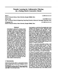
4.3. Experimental Results. It can be seen from (8) that 𝛼 and the number 𝐾 of neighbors with the most similar or most dissimilar interested trend have an inevitable influence on the performance of CFCM. In this section, we first evaluate the impact of 𝛼 and 𝐾 on the performance of CFCM, and then we compare CFCM with the state-of-the-art approaches based on traditional CF methods. We can find that at 𝛼 = 0, (8) degenerates to 𝑟̂ = 𝑟𝑢 + (∑V∈𝑈𝑢,𝑑 |𝑐𝑜V(𝑢, V)| × 𝑢𝑖 (𝑟V𝑖 − 𝑟V ))/ ∑V∈𝑈𝑢,𝑑 |𝑐𝑜V(𝑢, V)|, i.e., the calculation of 𝑟̂ 𝑢𝑖 only considers 𝐾 most dissimilar neighbors of the target user. Obviously, 𝛼 = 0 is a special case for our method. Figure 1 shows the impact of the parameters 𝛼 and 𝐾 on MAE. As shown in Figure 1, we can learn that when 𝛼 ≠ 0, MAE decreases with 𝛼 for any fixed K; i.e., the recommendation precision increases with 𝛼 for any fixed 𝐾. This result is not surprising because 𝛼 represents the weight of ensuring the recommended precision in (8), and a larger 𝛼 means a higher recommendation precision. Furthermore, we can find from Figure 1 that MAE remains relatively stable when 𝛼 is greater than 0.8 which means that there is much less benefit to improve the prediction precision of recommendation by continually increase 𝛼 when it is larger the 0.8. We can also observe that MAE decreases with 𝐾 when 𝛼 takes a fixed value between 0 and 0.7. This is because the larger 𝐾 means more neighbors are considered when calculating the rating prediction. The more neighbors naturally lead to the better recommendation precision. In addition, for a fixed 𝛼 between 0.7 and 1, MAE no longer decreases with 𝐾 when 𝐾 is greater than 20. This demonstrates when 𝛼 is greater than 0.7, the recommendation precision cannot be simply improved

6

Mathematical Problems in Engineering 0.225

0.67

0.22

0.65

0.215

0.63 F1

NMAE

0.21 0.205

0.61

0.2

0.59

0.195

0.57

0.19 0.185

0.55 0

0.2

0.4



0.6

0.8

0

0.2

1

K=20

K=40

K=60

K=60

K=100

Figure 2: Impact of 𝛼 and 𝐾 on NMAE.

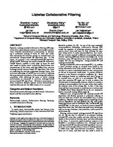
by increasing 𝐾. For 𝛼 = 0, the trend of MAE is slightly fluctuating only when 𝐾 is relatively small, such as 𝐾 = 20. At the same time, we find that 𝐾 had very little influence on MAE at 𝛼 = 0. Figure 2 demonstrates the impact of the parameters 𝛼 and 𝐾 on NMAE. As we expect, the result and the trend of the curve are very similar to Figure 1. The reason is that NMAE is the normalized MAE. Figure 3 depicts the impact of the parameters 𝛼 and 𝐾 on F1. We can see from Figure 3 that F1 increases with 𝛼 for any fixed K, that is, the recommendation comprehensive performance (including precision and recall) increases with 𝛼 for any fixed 𝐾. The reason is the same as the one for Figure 1. We can also observe from Figure 3 that F1 increases with 𝐾 when 𝛼 takes a fixed value between 0 and 0.7, and the growth rate gradually reduces as 𝛼 increases. When 𝛼 takes a fixed value between 0.7 and 1, F1 no longer increases with 𝐾. This demonstrates when 𝛼 is greater than a certain threshold (i.e., 0.7), it is not feasible to improve the recommendation comprehensive performance by increasing K. Figure 4 shows the impact of the parameters 𝛼 and 𝐾 on Diversity. We can find from Figure 4 that Diversity decreases with 𝛼 for any fixed K, and this decreasing trend becomes more apparent when 𝛼 is greater than 0.8. This result is not surprising because the increase of 𝛼 means the decrease of the weight that ensures the recommendation diversity. We can also observe from Figure 4 that Diversity has a very small change with 𝐾 when 𝛼 takes a fixed value between 0 and 0.9. This demonstrates that Diversity mainly depends on 𝛼 and is less affected by K.

0.6 

0.8

1

K=20

K=40 K=80

0.4

K=80 K=100

Figure 3: Impact of 𝛼 and 𝐾 on F1.

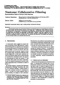
By analyzing Figures 1–4, we can find that when 𝛼 takes 0.8, CFCM can achieve the optimal overall performance in terms of both recommendation precision and recommendation diversity. Further, in order to demonstrate the superiority of CFCM, we compare CFCM with the existing CF methods based on the traditional similarity measures. In the state-ofthe-art CF methods, we select PCC [11], CPCC [12], JMSD [14], MJD [15], PIP [16], AC-PCC [17], NHSM [18], and BCF [19] as the baseline methods of our experiments. For CFCM, the parameter 𝛼 is set to 0.8 in the following experiments. To ensure fairness, we adopt the optimal experimental parameter setting for each baseline method. Figure 5 shows the performance comparison of CFCM with the above-mentioned eight methods on MAE for different 𝐾. As we expect, our method CFCM evidently outperforms the other eight methods on MAE at all 𝐾 values. We can also observe from Figure 5 that the MAE of CFCM is the most stable and is almost unaffected by 𝐾. The reason is that the user-user covariance matrix has a finer description capability for user similarity trend than the traditional similarity measures. Figure 6 depicts the performance comparison of CFCM with the other eight methods on NMAE for different 𝐾. As shown in Figure 6, CFCM evidently outperforms the other eight methods on NMAE at all 𝐾 values. Similar to Figure 5, the NMAE of CFCM is the most stable and is almost unaffected by K. Figure 7 demonstrates the performance comparison of CFCM with the other eight methods on F1 for different 𝐾.

Mathematical Problems in Engineering

7 0.25

0.9 0.85

0.24

0.8

0.23

0.75 NMAE

Diversity

0.7 0.65 0.6

0.22 0.21

0.55

0.2

0.5

0.19

0.45 0.4

0.18 0

0.2

0.4

0.6 

0.8

1

20

40

60

80

100

120

K PCC PIP CPC JMSD MJD NHSM

K=20 K=40 K=60 K=80

AC_PCC BCF CFCM

K=100

Figure 4: Impact of 𝛼 and K on Diversity.

Figure 6: Performance comparison on NMAE.

1 0.7 0.65

0.95

0.6 0.55

MAE

0.9

F1

0.5

0.85

0.45 0.4

0.8

0.35 0.3

0.75

20

40

60



80

PCC PIP CPC JMSD MJD NHSM AC_PCC BCF CFCM

Figure 5: Performance comparison on MAE.

100

0.25

20

40

60

80 K

PCC PIP CPC JMSD MJD NHSM AC_PCC BCF CFCM

Figure 7: Performance comparison on F1.

100

8

Mathematical Problems in Engineering 0.75

[20], to measure the proposed approach more comprehensively.

0.7 0.65

Data Availability

Diversity

0.6

The data used to support the findings of this study are available from the corresponding author upon request.

0.55 0.5

Conflicts of Interest

0.45

The authors declared no conflicts of interest regarding the submission of this manuscript.

0.4 0.35 0.3

Acknowledgments 20

40

60

K

80

100

PCC PIP CPC JMSD MJD NHSM AC_PCC BCF CFCM

Figure 8: Performance comparison on Diversity.

We can see from Figure 7 that CFCM evidently outperforms the other eight methods on F1 at all 𝐾 values. We can also observe from Figure 7 that the NMAEs of CFCM, NHSM and AC PCC are almost unaffected by 𝐾 and have a good stability. Figure 8 shows the performance comparison of CFCM with the other eight methods on Diversity for different 𝐾. As we expect, CFCM evidently outperforms the other eight methods on Diversity at all 𝐾 values. This is because CFCM adds the influencing factor from the neighbors with the most dissimilar interested trend into the rating prediction, which enhances the diversity of recommendation results.

5. Conclusion Although the traditional CF methods have been widely studied and deployed, most of these methods suffer several inherent weaknesses. In this paper, to solve the inherent weaknesses we build a new user-user covariance matrix to replace the traditional CF’s user-user similarity matrix. Compared to the user-user similarity matrix, the user-user covariance matrix has a finer description capability for user similarity trends, and especially for the users without common rated items, it shows the more powerful description capability. Further, we propose an enhancing collaborative filtering method based on the user-user covariance matrix. The experimental results show that the proposed method can significantly improve the diversity of recommendation results in ensuring a good recommendation precision. In the future work, we will consider introducing new quality measure metrics, such as coverage quality measure

This work is supported by the National Nature Science Foundation of China (61702368 and 61170174), Major Research Project of National Nature Science Foundation of China (91646117), Natural Science Foundation of Tianjin (17JCYBJC15200, 15JCYBJC46500, and 18JCQNJC00700), and the Opening Foundation of Tianjin Key Laboratory of Intelligence Computing and Novel Software Technology (TJUTKLICNST-K20170001).

References [1] Y. Xiao, G. Wang, C. Hsu, and H. Wang, “A time-sensitive personalized recommendation method based on probabilistic matrix factorization technique,” Soft Computing, vol. 22, no. 20, pp. 6785–6796, 2018. [2] D. Goldberg, D. Nichols, B. M. Oki, and D. Terry, “Using collaborative filtering to weave an information tapestry,” Communications of the ACM, vol. 35, no. 12, pp. 61–70, 1992. [3] T. Hofmann, “Collaborative filtering via gaussian probabilistic latent semantic analysis,” in Proceedings of the 26th International ACM SIGIR Conference on Research and Development in Informaion Retrieval (SIGIR), pp. 259–266, Toronto, Canada, 2003. [4] T. Hofmann, “Latent semantic models for collaborative filtering,” ACM Transactions on Information and System Security, vol. 22, no. 1, pp. 89–115, 2004. [5] A. Kohrs and B. Merialdo, “Clustering for collaborative filtering applications,” in Proceedings of the International Conference on Computational Intelligence for Modelling, Control and Automation, 1999. [6] J. D. M. Rennie and N. Srebro, “Fast maximum margin matrix factorization for collaborative prediction,” in Proceedings of the 22nd International Conference on Machine Learning (ICML ’05), pp. 713–719, August 2005. [7] R. Salakhutdinov and A. Mnih, “Bayesian probabilistic matrix factorization using markov chain Monte Carlo,” in Proceedings of the 25th International Conference on Machine Learning (ICML ’08), pp. 880–887, ACM, Helsinki, Finland, July 2008. [8] Y. Xiao, P. Ai, C.-H. Hsu, H. Wang, and X. Jiao, “Time-ordered collaborative filtering for news recommendation,” China Communications, vol. 12, no. 12, pp. 53–62, 2015. [9] G. Linden, B. Smith, and J. York, “Amazon.com recommendations: item-to-item collaborative filtering,” IEEE Internet Computing, vol. 7, no. 1, pp. 76–80, 2003. [10] P. Resnick, N. Iacovou, M. Suchak, P. Bergstrom, and J. Riedl, “GroupLens: An open architecture for collaborative filtering

Mathematical Problems in Engineering

[11]

[12]

[13]

[14]

[15]

[16]

[17]

[18]

[19]

[20]

of netnews,” in Proceedings of the 1994 ACM Conference on Computer Supported Cooperative Work, CSCW 1994, pp. 175– 186, USA, October 1994. M. D. Ekstrand, J. T. Riedl, and J. A. Konstan, “Collaborative filtering recommender systems,” ACM Transactions on Information Systems, vol. 4, no. 2, pp. 81–173, 2011. U. Shardanand and P. Maes, “Social information filtering: algorithms for automating ‘word of mouth’,” in Proceedings of the Conference on Human Factors in Computing Systems, pp. 210– 217, May 1995. F. Cacheda, V. Carneiro, D. Fern´andez, and V. Formoso, “Comparison of collaborative filtering algorithms: Limitations of current techniques and proposals for scalable, high-performance recommender systems,” ACM Transactions on the Web (TWEB), vol. 5, no. 1, pp. 1–33, 2011. J. Bobadilla, F. Serradilla, and J. Bernal, “A new collaborative filtering metric that improves the behavior of recommender systems,” Knowledge-Based Systems, vol. 23, no. 6, pp. 520–528, 2010. J. Bobadilla, F. Ortega, A. Hernando, and J. Bernal, “A collaborative filtering approach to mitigate the new user cold start problem,” Knowledge-Based Systems, vol. 26, pp. 225–238, 2012. H. J. Ahn, “A new similarity measure for collaborative filtering to alleviate the new user cold-starting problem,” Information Sciences, vol. 178, no. 1, pp. 37–51, 2008. P. Pirasteh, D. Hwang, and J. E. Jung, “Weighted Similarity Schemes for High Scalability in User-Based Collaborative Filtering,” Mobile Networks and Applications, vol. 20, no. 4, pp. 1–11, 2014. H. Liu, Z. Hu, A. Mian, H. Tian, and X. Zhu, “A new user similarity model to improve the accuracy of collaborative filtering,” Knowledge-Based Systems, vol. 56, pp. 156–166, 2014. B. K. Patra, R. Launonen, V. Ollikainen, and S. Nandi, “A new similarity measure using Bhattacharyya coefficient for collaborative filtering in sparse data,” Knowledge-Based Systems, vol. 82, pp. 163–177, 2015. J. Bobadilla, F. Ortega, A. Hernando, and A. Guti´errez, “Recommender systems survey,” Knowledge-Based Systems, vol. 46, pp. 156–166, 2013.

9

Advances in

Operations Research Hindawi www.hindawi.com

Volume 2018

Advances in

Decision Sciences Hindawi www.hindawi.com

Volume 2018

Journal of

Applied Mathematics Hindawi www.hindawi.com

Volume 2018

The Scientific World Journal Hindawi Publishing Corporation http://www.hindawi.com www.hindawi.com

Volume 2018 2013

Journal of

Probability and Statistics Hindawi www.hindawi.com

Volume 2018

International Journal of Mathematics and Mathematical Sciences

Journal of

Optimization Hindawi www.hindawi.com

Hindawi www.hindawi.com

Volume 2018

Volume 2018

Submit your manuscripts at www.hindawi.com International Journal of

Engineering Mathematics Hindawi www.hindawi.com

International Journal of

Analysis

Journal of

Complex Analysis Hindawi www.hindawi.com

Volume 2018

International Journal of

Stochastic Analysis Hindawi www.hindawi.com

Hindawi www.hindawi.com

Volume 2018

Volume 2018

Advances in

Numerical Analysis Hindawi www.hindawi.com

Volume 2018

Journal of

Hindawi www.hindawi.com

Volume 2018

Journal of

Mathematics Hindawi www.hindawi.com

Mathematical Problems in Engineering

Function Spaces Volume 2018

Hindawi www.hindawi.com

Volume 2018

International Journal of

Differential Equations Hindawi www.hindawi.com

Volume 2018

Abstract and Applied Analysis Hindawi www.hindawi.com

Volume 2018

Discrete Dynamics in Nature and Society Hindawi www.hindawi.com

Volume 2018

Advances in

Mathematical Physics Volume 2018

Hindawi www.hindawi.com

Volume 2018