Abstract
Presentation
Paper
Table Paper of Contents
ASAP 2001 Proceedings
Next Abstract
Covariance Matrix Filtering for Adaptive Beamforming with Moving Interference Bruce K. Newhall Johns Hopkins University Applied Physics Laboratory 11100 Johns Hopkins Road Laurel, MD 20723-6099
[email protected]
ABSTRACT An approach is developed for adaptive beamforming for mobile sonars operating in an environment with moving interference from surface shipping. It is assumed that the sound source of each ship is drawn from an ensemble o f Gaussian random noise, but each ship moves at constant speed along a deterministic course. An analytic expression for the ensemble mean covariance is obtained. In practice the location, course, speed, mean noise level, and transmission loss of each interferer are not known with sufficient precision to use the modeled ensemble mean as a basis for adaptive beamforming. The problem is thus t o accurately estimate the ensemble mean based on data samples. The analytic ensemble mean is not stationary, and thus is not well estimated by the sample mean. The ensemble of covariance samples consists of rapidly varying random terms associated with the emitted noise and more slowly oscillating deterministic terms associated with the source and receiver motion. The non-stationary ensemble covariance mean can be estimated by filtering out the rapidly varying noise while retaining the slow oscillatory terms. Performance of the filters can be visualized and assessed in the "epoch” frequency domain, the Fourier transform of the covariance samples. In this domain, higher bearing rates show up at higher frequencies. The traditional sample mean estimator retains only the zerofrequency bin corresponding to stationary interference. Techniques that can identify and include the appropriate non-zero frequency contributions are better non-stationary estimators than the sample mean. Several such techniques are offered and compared. Simulations are invaluable i n evaluating the filter performance, since the ensemble mean can be precisely calculated analytically in the simulation, and compared directly with the sample estimates. Simulations of adaptive beamformers using covariance filtering will be shown to yield improved robustness t o shipping motion.
1.
INTRODUCTION
At low frequencies, underwater noise is dominated by shipping sources. These sources can be extremely loud, and can dominate the performance of low-frequency passive sonar systems. Since these sources are typically spatially discrete, adaptive techniques ought to apply to eliminate their influence when surveillance is performed in locations in between the loud ships. Unfortunately, the
shipping sources are moving, and hence violate the stationary noise assumptions of current adaptive techniques. Current implementations of adaptive beamformers often do not achieve much gain above conventional, non-adaptive beamformers and hence remain limited by the loud sources of interference. Here we suggest a new class of techniques that may robustly achieve the rejection of loud sources of moving interference.
2.
PHYSICAL MODEL OF SHIPPING NOISE
Current adaptive techniques are based on the physical assumption that the sources of interference are stationary in space. This is clearly not valid for the case of moving ocean shipping sources. Hence, we must develop a new physical model for the interference in order to derive the appropriate adaptive processing.
2.1
Pressure Field
Begin by assuming an arbitrary set of ships under deterministic motion in an arbitrary underwater sound channel. We focus on a single frequency, with the assertion that the model can be extended to the broadband case by a straightforward summation across frequencies. In the selected frequency bin, it is reasonable to model the sound source of each ship by a draw from an ensemble of complex Gaussian random noise, and assume that the noises of different ships are fundamentally independent. These sources are then propagated to each receiver array element. The propagation may be described by a coherent sum over modes [1]. In a range independent environment, these modes arise naturally with the use of a normal mode propagation model. In range-dependent environments, the propagation can be expanded as a sum of local modes in the vicinity of the receiver. This local mode expansion is explicit via the use of coupled or adiabatic mode propagation models, but in principle can be obtained from the field output of any propagation modeling technique. The received acoustic pressure pn at the nth element in an array is a sum across ships of the sum over the local modes:
Form Approved OMB No. 0704-0188
Report Documentation Page
Public reporting burden for the collection of information is estimated to average 1 hour per response, including the time for reviewing instructions, searching existing data sources, gathering and maintaining the data needed, and completing and reviewing the collection of information. Send comments regarding this burden estimate or any other aspect of this collection of information, including suggestions for reducing this burden, to Washington Headquarters Services, Directorate for Information Operations and Reports, 1215 Jefferson Davis Highway, Suite 1204, Arlington VA 22202-4302. Respondents should be aware that notwithstanding any other provision of law, no person shall be subject to a penalty for failing to comply with a collection of information if it does not display a currently valid OMB control number.
1. REPORT DATE
2. REPORT TYPE
14 MAR 2001
N/A
3. DATES COVERED
-
4. TITLE AND SUBTITLE
5a. CONTRACT NUMBER
Covariance Matrix Filtering for Adaptive Beamforming with Moving Interference
F19628-00-C-0002 5b. GRANT NUMBER 5c. PROGRAM ELEMENT NUMBER
6. AUTHOR(S)
5d. PROJECT NUMBER
Bruce K. Newhall
5e. TASK NUMBER 5f. WORK UNIT NUMBER
7. PERFORMING ORGANIZATION NAME(S) AND ADDRESS(ES)
Johns Hopkins University Applied Physics Laboratory 11100 Johns Hopkins Road Laurel, MD 20723-6099 9. SPONSORING/MONITORING AGENCY NAME(S) AND ADDRESS(ES)
8. PERFORMING ORGANIZATION REPORT NUMBER
10. SPONSOR/MONITOR’S ACRONYM(S) 11. SPONSOR/MONITOR’S REPORT NUMBER(S)
12. DISTRIBUTION/AVAILABILITY STATEMENT
Approved for public release, distribution unlimited 13. SUPPLEMENTARY NOTES
See ADM001263 for entire Adaptive Sensor Array Processing Workshop. 14. ABSTRACT
An approach is developed for adaptive beamforming for mobile sonars operating in an environment with moving interference from surface shipping. It is assumed that the sound source of each ship is drawn from an ensemble of Gaussian random noise, but each ship moves at constant speed along a deterministic course. An analytic expression for the ensemble mean covariance is obtained. In practice the location, course, speed, mean noise level, and transmission loss of each interferer are not known with sufficient precision to use the modeled ensemble mean as a basis for adaptive beamforming. The problem is thus to accurately estimate the ensemble mean based on data samples. The analytic ensemble mean is not stationary, and thus is not well estimated by the sample mean. The ensemble of covariance samples consists of rapidly varying random terms associated with the emitted noise and more slowly oscillating deterministic terms associated with the source and receiver motion. The non-stationary ensemble covariance mean can be estimated by filtering out the rapidly varying noise while retaining the slow oscillatory terms. Performance of the filters can be visualized and assessed in the "epoch frequency domain, the Fourier transform of the covariance samples. In this domain, higher bearing rates show up at higher frequencies. The traditional sample mean estimator retains only the zerofrequency bin corresponding to stationary interference. Techniques that can identify and include the appropriate non-zero frequency contributions are better non-stationary estimators than the sample mean. Several such techniques are offered and compared. Simulations are invaluable in evaluating the filter performance, since the ensemble mean can be precisely calculated analytically in the simulation, and compared directly with the sample estimates. Simulations of adaptive beamformers using covariance filtering will be shown to yield improved robustness to shipping motion. 15. SUBJECT TERMS
16. SECURITY CLASSIFICATION OF: a. REPORT
b. ABSTRACT
c. THIS PAGE
unclassified
unclassified
unclassified
17. LIMITATION OF ABSTRACT
18. NUMBER OF PAGES
UU
5
19a. NAME OF RESPONSIBLE PERSON
Standard Form 298 (Rev. 8-98) Prescribed by ANSI Std Z39-18
pn = ∑ ∑ s j Amn (t )e j
ikm r jn ( t )
m
where s j is the source noise sample, Amn is the mode amplitude and k m is the wavenumber of the mth mode, and rjn is the range from the jth ship to the nth receiver element. Note that the mode amplitudes must incorporate cylindrical spreading and attenuation terms not given explicitly here. The pressure consists of random contributions from the ship noise sources and deterministic time-varying propagation contributions.
2.2
Covariance
Optimal adaptive processing is determined from the mean of the covariance among sensor pressures. This expectation must be taken across the random ensemble of ship sources. The ensemble-mean covariance will be a function of time because of the time varying propagation terms. Therefore the expected covariance cannot be obtained directly from a sample mean across time samples of the covariance. Using the independence of different ships an analytic expression for the ensemble covariance is obtained:
pn1 p n2 * =
ΣΣΣ j
× Am1n1 A m2 n2 e
(
m1
sj s j *
m2
i k m rjn ( t ) −k m r jn ( t) 1
1
2
2
)
where the brackets indicate the expectation across the ensemble. The term is the power spectrum of the jth source. If the ranges, propagation modes, and source level power spectra were all known, this model expression could be calculated at each time and used in a standard minimum variance distortionless response (MVDR) full-rank ABF [2, 3]. This approach might be termed the full knowledge a priori model-based MVDR method. Such an ABF would move its nulls in time to optimally reject noise from all the moving ships. Unfortunately, it is unlikely in practice that full knowledge will be available a priori. Precisely predicting the propagation structure is quite difficult given the spatial and temporal variability of the ocean. It is also unlikely that the exact source power spectra will be known for every contributing ship. Thus, we usually must attempt to estimate the unknowns in the ensemble mean covariance from data samples.
oscillatory nature of the exponential terms will produce a sample mean that tends to zero over long estimation times, while the ensemble mean is significantly larger. To avoid underestimating the ensemble mean, alternatives to the sample mean are considered.
3.1 Fourier Analysis and Synthesis An alternative to sample averaging is to apply fourier analysis to covariance samples. One motivation for this approach is to separate the differing time scales involved. The random source noise varies rapidly from one sample to the next. This rapid variation produces a sample noise that is nearly white. This sample noise will corrupt estimates of the ensemble mean covariance unless it is removed. The deterministic amplitudes and phases from the propagation terms vary more slowly and continuously in time. A low pass filter is expected to separate the rapidly varying sample noise from the slowly varying propagation terms. Since filter behavior is often best analyzed in the frequency domain, this motivates transforming the covariance samples to a corresponding frequency domain. This domain will be referred to as the epoch frequency domain to distinguish it from the acoustic frequency. A second motivation for considering the Fourier transform of the covariance samples can be obtained by considering the time dependence of the propagation terms. The propagation amplitudes typically evolve very slowly in time, and this variation made be neglected for the moment. The most rapidly changing term is the phase term due to the changing ranges to the interference sources. Expand the ranges in a Taylor series about some reference time:
r = r0 + r&t + ... where r0 is the range at the reference time t=0 and r& is the initial range rate of the source. Again for the moment, higher order terms will be neglected. The ensemble covariance can now be approximated by
p n1 p n2 * = Σ Σ Σ j
ALGORITHMS
Since the ensemble mean involves deterministic timevarying terms, it cannot be reliably estimated directly from a sample mean taken over time. In particular, the
m1 m 2
× e i (km1 r jn1 0 −km 2 r jn2 0 )e i (km1r&jn1 −km 2 r&jn2 )t In this form, the unknowns: source power spectra and propagation amplitudes are coefficients of sinusoidal complex exponentials with epoch frequencies Ω = k m r&jn − k m r&jn
3.
s j s j * Am1n1 Am2 n2
1
1
2
2
. This suggests that these unknown
coefficients can be estimated by Fourier analysis. Once the coefficients are estimated then the original time series for the ensemble covariance is reconstructed via Fourier synthesis.
The overall approach is summarized as follows. First obtain time samples of the elements of the covariance matrix, as is currently done in ABF. For each matrix element, transform the time samples of covariance to the epoch frequency domain. Identify the appropriate frequencies associated with the moving ships, and use those frequency coefficients to synthesize the ensemble mean time series. The only portion of the algorithm remaining to specify is the technique of identifying which frequencies in the epoch domain are associated with the shipping noise sources and which are dominated by sample noise. Several methods can be employed.
3.2 Covariance Low-pass Filtering Methods Since ships generally do not change range significantly within a few time samples, the shipping noise is expected to nearly always occur in the lowest frequency bins of the epoch frequency domain, while sample noise is expected to be nearly white across all bins. Hence, appropriate low pass filters are expected to retain much of the shipping noise energy to be estimated, while rejecting the sample noise. The best selection of pass band is made based on the expected motion of the contributing ships. Current ABF algorithms that employ the sample mean are in fact an example of covariance low pass filtering, since the sample mean is the low pass filter that retains only the spectral power in the zero-frequency bin. The performance of any low pass filter can be improved by matching the filter width to the expected epoch frequency widths associated with typical ship motion. For rapidly moving ships, this can be achieved by retaining more frequency bins in the filter. In order to further improve over current algorithms, advantage must be taken of the specifics of the epoch frequency structure of the shipping noise. The epoch frequency for each ship given above depends of the difference of the products of a wavenumber times a range rate. Underwater acoustic wavenumbers of the significant modes generally do not exhibit much spread. Furthermore, for operational horizontal line arrays, the interfering ships will almost always occur at ranges significant relative to the horizontal separation between array elements. In these cases the epoch frequency where a ship contributes can be approximated by
Ω ≈ k 0 ∆xθ sin θ where k0 is a reference wavenumber, ∆x is the horizontal separation between elements, θ is the bearing to the ship θ (relative to the line between the elements), and is the bearing rate. Note that the epoch frequency increases approximately linearly with separation between elements. This suggests a second filtering approach, in which the low pass filter frequency width is increased linearly proportionally to separation. Elements near the main
diagonal of the covariance matrix are less affected by source motion, and hence can be estimated with narrower low-pass filters. The most separated elements at the farthest corners of the matrix are the most subject to source motion, and require the highest bandwidth low-pass filter. The maximum bandwidth can be selected to match the highest bearing rate typically encountered.
3.2 Covariance Band-pass Filtering Methods Further improvements in estimation may be potentially obtained by retaining only those epoch frequency bins containing significant shipping noise. One method involves partial knowledge available a priori. When the locations and tracks of the significant ships are independently known, for example from radar surveillance, then the bearing rates can be calculated and the epoch frequency bins identified. The energy in the identified bins then represents estimates of the unknown propagation and source level terms. Fourier synthesis using only the identified bins produces the desired covariance time series. The entire process can be described as a set of band pass filters, where each narrow pass band is selected based on the knowledge a priori of the bearing rates. When no knowledge is available a priori, the potential exists to take advantage of the linear dependence on separation. Energy from each individual ship will lie along a line in the separation-epoch frequency plane. Line detection methods in this plane have the potential to automatically identify the appropriate bearing rates associated with significant interfering energy. Such methods may include Radon or Hough transforms [4]. Once the appropriate bins have been identified, band pass filters can be constructed to filter the shipping noise from the sample noise.
4.
SIMULATION
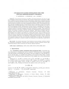
A simulation was performed to demonstrate the potential utility of these techniques. In the simulation, the exact ensemble mean can be calculated since all quantities are known. Adaptive processing based on this exact mean covariance gives an upper bound to the maximum performance that could be achieved, if, for example, perfect knowledge were available a priori. In addition to the ensemble mean, the simulation generated time samples of covariance from four moving ships with Gaussian noise sources. The ships were moving at realistic speeds from between 10 and 20 knots. The tracks of the ships are shown in figure 1. Noise from the ships was propagated with cylindrical spreading in a single mode underwater channel. The noise was received on a line array of 50 elements with a design frequency of 60 Hz. The simulation was performed at this design frequency.
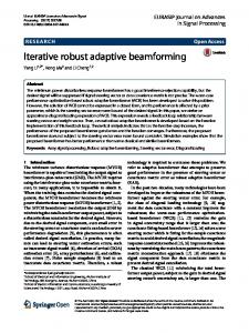
The sample mean ABF performed almost no better than conventional non-adaptive ABF in the simulation. The sample mean was unable to properly capture the motion of the ships, and hence was unable to place nulls in the proper locations to cancel the ship noise. The element dependent ABF filtered sample covariance showed a median improvement of about 5 dB reduction in the noise over the sample mean approach. The perfect ensemble mean displayed 10 dB reduction in noise beyond the sample mean method.
12
Range (km)
8 4 0 -4
5. -10
-5
0 5 Range (km)
1 0
1 5
Figure 1. Tracks of the four ships in the simulation relative to array at origin The simulation calculated the conventional beamformer response and compared with various MVDR beamformer responses for a set of beams spanning all azimuths. The beamformers used various estimates of the ensemble mean covariance. In addition to the exact ensemble mean, the ABF based on the sample mean and the ABF based on an element dependent low-pass filter were simulated. Results of the simulation are summarized by cumulative distributions of noise across all beams shown in figure 2.
1 ABF mean
Probability
0. 8
ensemble
ABF filtered sample estimation
0. 6 0. 4
ABF sample mean
0. 2 0
CBF 0
60 0 40 30 Relative Beam Noise Level
20
Figure 2. Cumulative distributions of noise for various beamformers
CONCLUSIONS
The problem of adapting in the presence of moving sources of interference was considered. Application was particularly addressed to the motion of interfering surface ship noise for passive sonar arrays. The physics of ship motion was modeled, including the received noise field and the noise covariance matrix. An analytic expression of the ensemble mean covariance was obtained. This physical model suggested a new approach of covariance filtering to better estimate the ensemble mean covariance from data samples. Two paradigms of current adaptive beamforming may need to be abandoned in the presence of interference motion. First, the sample mean may not be the appropriate estimator when the interference sources are in motion. Second, the covariance matrix may not be treated as a single entity, since motion affects different elements of the matrix differently. The behavior of the covariance under interference motion can be visualized in the epoch frequency domain. This domain is the Fourier transform of the samples of the covariance matrix. It was observed that energy from each moving ship falls along an approximate line in the epoch frequency / element separation plane. Several methods for obtaining improved estimates of the ensemble mean covariance were suggested. Preliminary investigations of relative performance of a few of these methods were obtained via a simulation. Much remains to be done to develop these methods further. There is great potential for refinement of the algorithms and development of better filtering techniques. The epoch frequency domain has only begun to be explored. Line detection techniques have yet to be attempted. It has been suggested that the covariance matrix may also have a near-toeplitz structure in the epoch frequency domain [5]. If so, then toeplitz averaging, or low-pass filtering along the toeplitz directions may provide additional rejection of sample noise. Finally, applications of this class of techniques to real data are certainly warranted.
Abstract
Presentation
Paper
Table Paper of Contents
Next Abstract 6.
REFERENCES
[1] C.A. Boyles, Acoustic Waveguides Application to Oceanic Science, Wiley Interscience, New York, 1984, p. 174. [2] J.N. Maksym, “A robust formulation of an optimum cross-spectral beamformer for line arrays,” J. Acoustic. Soc. Am., vol. 65, no. 4, Apr. 1979, pp. 971-975. [3] J. Capon, “High-Resolution Frequency-Wavenumber Spectrum Analysis,” Proceedings of the IEEE, vol. 57, no. 8, Aug. 1969, pp. 1408-1418. [4] J. Illingworth and J. Kittler, “A Survey of the Hough Transform,” Computer Vision, Graphics and Image Processing, vol. 44, no. 1, 1988, pp. 87-116. [5] R. Pitre, personal communication.