984. Enhancing Modularity-Based Graph Clustering. Azzam Sleit, Sawsan Abusharkh and Wesam AlMobaideen. University of Jordan, P.O. Box 13898, Amman ...
World Applied Sciences Journal 9 (9): 984-996, 2010 ISSN 1818-4952 © IDOSI Publications, 2010
Enhancing Modularity-Based Graph Clustering Azzam Sleit, Sawsan Abusharkh and Wesam AlMobaideen University of Jordan, P.O. Box 13898, Amman 11942, Jordan Abstract: Graph clustering is defined as grouping the vertices of a given input graph into clusters. This article proposes a Two-Phase Modularity-Based Graph Clustering (2-PMGC) algorithm based on modularity optimization. The algorithm consists mainly of two steps; namely, coarsening and refinement. The coarsening phase takes the original graph as input and produces levels of coarsen graphs. The second phase starts with the coarsest graph resulting from the previous phase and enhances clustering by further moving the vertices of each coarsen level between clusters. Our algorithm is evaluated for 16 real-world networks, where an obvious increase in modularity is achieved by the proposed algorithm. Key words: Graph Clustering
Modularity
Community Detection
INTRODUCTION Graph clustering (GC) is defined as the process of separating an input graph into sub-graphs called clusters. Graph clustering algorithms have gained much attention recently, in various areas, such as data mining, statistics, biology and computer networks. The problem of communities’ detection can be modelled as a graph clustering process, where vertices correspond to individual items, edges describe relationships and clusters correspond to communities [1]. To evaluate the goodness of clustering algorithms, an objective function must be determined. Modularity is a benefit function which was first introduced by Newman and Girvan [2]. It is based on the idea that a graph has community structure if it is not a random graph. In random graphs, every two vertices have the same probability to be adjacent [3]. Modularity is defined as follows [4].
(
1 Q = Σij Aij − Pij 2m
) (Ci ,C j )
(1)
is the adjacency matrix, is the total number of edges of the graph and represents the expected number of edges between vertices and in the null model. (ci is a function defined as: c =c (2) 1 i j ( c =c ) = i j 0
otherwise
The choice of the null model has several possibilities, in the standard null model, the probability that vertex with
Greedy Algorithm
degree can be connected to a vertex with degree can be calculated easily [3]. The probability to choose randomly an edge incident with vertex is ki, since there are edges incident with out of a total of. Then, the probability of forming an edge between and is l. The expected number is Pij = 2m pi pj = kikj. The modularity of a graph can be calculated as follows. Q =
1 2m
∑ ij Aij −
ki k j (Ci ,C j ) 2m
(3)
The modularity is not only used as a quality function to clustering, but it is used in the analysis of networks or graphs such as computer or social networks. It has shown its relevance in solving the problem of extracting dense clusters in a graph. Modularity optimization is a problem that is computationally hard [2]. Therefore, approximation algorithms are necessary when dealing with large networks. Depending on desirable structure of the clusters, graph clustering algorithms can be classified into two paradigms; namely, hierarchical and flat clustering [4]. Hierarchical clustering produces multi-level clustering, where the resulting clusters can be modeled as a tree called Dendrogram. This is accomplished by iterating partitions, in which the root cluster almost contains the whole vertices and the leaf clusters contains at least one vertex. Flat clustering generates sub-graphs; each contains vertex subset from the whole graph. When the final number of clusters is known beforehand, flat clustering is more efficient.
Corresponding Author: Azzam Sleit, University of Jordan, P.O. Box 13898, Amman 11942, Jordan 984
World Appl. Sci. J., 9 (9): 984-996, 2010
Fig. 1: Agglomerative Clustering Furthermore, the Hierarchical Graph Clustering Can Be Classified Into:
connected by an edge in the original graph such that the modularity increases. Clauset, et al. [9] proposed a bottom-up greedy optimization algorithm to maximize the modularity of graph clustering. The algorithm starts with singleton clusters in the input graph. Then, it finds the pair of clusters with the maximum modularity gain and then merges them. During the merge process, the algorithm updates the modularity gain values that correspond to any neighboring clusters of the newly merged ones. A multi-step greedy (MSG) algorithm by Schuetz and Caflish [10] was proposed. It depends on the greedy merging of more than one cluster pair at each iteration. The motive of this approach is to resolve the problem of premature concentration into few large clusters. It is found by Noak and Rotta [11] that this multi-step coarsening algorithm is no improvement over simple single-step coarsening for the modularity criteria. They utilized a refinement algorithm, in which single vertices are moved to the neighbouring cluster that yields the maximum increase in modularity [12]. Blondel, et al. [13] used a local search heuristic method to optimize the modularity problem of graph clustering. The basic method consists of a sequence of two iterative steps. The first step consists of sequentially moving the vertex to a cluster where the modularity gain is maximized. In the second step, a new graph is formed from the obtained clusters in the first step. The two steps are sequentially repeated and the process stops when there is no modularity gain. The drawback of this algorithm is that the accuracy of the resulting clusters is tested only on the final partition. Extremal optimization is a heuristic search proposed to achieve accuracy comparable with simulated annealing. This technique was used for modularity optimization by Duch and Arenas [14]. The algorithm starts with a random bi-partition of the network into two communities. Then, it moves vertices with the lowest fitness from one cluster to the other until no further increase in modularity is possible. The process is repeated recursively for each resulting partition.
Top-down (divisive approach) - this approach iteratively partitions the graph into clusters. Each level is typically divided into two sets or more. There are various techniques to split the graph, such as Cuts, Spectral methods, Betweenness, Markov chains and Random walks. Bottom-up (agglomerative approach) - this approach assigns each vertex to a cluster and repeatedly merges pairs of clusters till agglomerative tree is formed [5]. Most merging criterion is based on greedy optimization of the objective function. Fig. 1 shows a set of vertices and the corresponding dendrogram. Graph clustering generates application-specific output. In the field of social networks, clustering helps in the of analysis social interactions between people. Han and Yan proposed fuzzy clustering for social annotations which allows users to annotate web resources more easily, openly and freely than do taxonomies and ontologies [6]. Lee et al. used text-mining methodology to explore the development and features of digital library represented using graph [7]. In the field of bioinformatics, graph clustering is applied to classify the gene expression and protein interactions. Related Work: The problem of graph clustering has been studied in the last decades. Consequently, the literature is rich with several approaches for measuring quality of clustering. Modularity is considered the most used and best-known quality function so far [3]. In the following subsection, a number of different graph clustering methods is presented. Modularity-based Graph Clustering Algorithms: Newman proposed a greedy modularity-based graph clustering algorithm to maximize the modularity [8]. It is an agglomerative hierarchical method, which starts with a number of clusters. Iteratively, the number of clusters is decreased by one by merging two clusters that are 985
World Appl. Sci. J., 9 (9): 984-996, 2010
homogeneous clusters (the vertices of one cluster have the same attributes) using a unified distance measure [18]. Saha and Mitra [19] introduced an incremental graph clustering algorithm, which considers the dynamicity of the input graph. The algorithm can handle the topological changes of the input graph (representing a network). It uses the min-cut as the quality measure of the resulting clusters [20]. Graph Partitioning: Hierarchical graph clustering can be considered as a sibling for multilevel graph partitioning [15]. It consists of three phases: coarsening, partitioning and refinement (or uncoarsening). Kernighan and Lin proposed one of the earliest methods to solve the problem of partitioning electronic circuits onto boards [12]. The algorithm was also used to optimize the modularity function representing the difference between the number of edges inside the clusters and the number of edges lying between them. The algorithm iteratively performs the globally best vertex move such that each vertex is moved once without the restriction that the move should increase modularity [11]. The run-time and storage requirements increase rapidly with the number of clusters [3]. Fiduccia and Mattheyses proposed a linear-time iterative heuristic algorithm which starts with a possibly random solution and changes the solution by a sequence of moves, which are organized by multiple passes [21].
Fig. 2: The Block Diagram of the 2-PMGC Input: Original Graph //coarsening phase coarsestGraph Coarsening (originalGraph); init Cluster coarsest Graph; //Refinement Phase Clusters Uncoarsen And Refinement (initCluster);
Fig. 3: The 2-PMGC Algorithm Some algorithms that use the spectral properties for the graph to extract the clusters were proposed. This is achieved by using a mathematical representation of the graph based on computing the Eigen values or the Laplacian transform of the adjacency matrix of the graph [15]. A spectral clustering algorithm by White and Smyth was proposed to find the relationship between network communities and vector clusters, by first embedding the graph into a Euclidean space and then clustering the vectors by applying K-means clustering algorithm [16]. The main drawback of spectral methods is that they are computationally expensive for large graphs.
Proposed Graph Clustering Algorithm: Modularity is one of the most widely used quality measures for graph clustering. In this section, a 2-Phase Modularity-based Graph Clustering algorithm (2-PMGC) is introduced to enhance the modularity of graph clustering. The algorithm consists of two phases; namely, coarsening and refinement. Fig. 2 shows the block diagram of the basic operations of the 2-PMGC algorithm. In the first phase, the Louvain method [13] is adopted. This coarsening phase takes the original graph as an input and produces levels of coarsen graphs. The last level of coarsen graphs (coarsest) is used as the initial clustering for the following refinement phase. The second phase starts with initial solution and tries to find a better one in terms of modularity by further moving the vertices of each level between clusters. Further description for the algorithm is shown in Fig. 3. A refining phase usually starts with initial solution and attempts to find a better one. During the coarsening phase, a sequence of smaller graphs is produced. Each graph has fewer vertices than the previous ones. Thus, the input graph G1 is transformed into levels of smaller graphs G2, G3, G4…, Gm; i.e. |G1(V)| > |G2(V)| > …> |Gm(V)|. In this phase, a set vertices from a graph Gi can be combined
Other Graph clustering Algorithms: Van Dongen proposed a random-walk Markov-based clustering algorithm [17]. The algorithm converts the input graph into a Markov graph and then random walk operations are applied to eliminate the inter-cluster interactions. Markov chain is a stochastic process which produces a transition matrix that contains the probabilities of moving from the current state to another state. Newman and Girvan algorithm [2] is a divisive clustering technique based on the concept of edge betweenness centrality, which is a measure of the proportion of shortest paths between nodes that pass through a particular link. The algorithm was shown to perform well on a variety of graph clustering tasks, but its complexity can severely limit its applicability. Graph clustering algorithms are categorized depending on the topological structure of the resulting clusters. However, most of them ignore the properties of the vertices. Zhou, et al. proposes a novel graph clustering algorithm, which partitions the graph into 986
World Appl. Sci. J., 9 (9): 984-996, 2010
together to form a single vertex in the next level graph Gi+1. nc 1 1 To start the refinement phase, an initial solution = is ( ( ki (ci ,c ) ki ) (c j ,c)) Q lc − m 2 needed. This initial solution is the clustering found in the = (2m)2 c 1= c 1 i j previous coarsening phase. In this case, the coarsest graph is selected. In the uncoarsening phase, the nc nc 1 1 clustering of Gm is projected back to the original graph G1 = Q lc − dc2 2m 2 by going through intermediate graph levels Gm-1, Gm(2m) c 1= c 1 = 2 ….G1. At each level of uncoarsening, some finer optimizations are applied on the graph. In general, nc 2 l 1 refinement algorithms move vertices between clusters, in dc Q ( c − = ) 2m 2m 2m order to improve the quality of the clustering. The c =1 technique for moving vertices is based on the FiducciaMattheyses (FM) refinement algorithm [21]. Where: The modularity as defined in Eq. (3) is a scalar value is the sum of internal edges of each cluster and between -1 and 1, which measures the density of links is the sum of the edges incident to the vertices in inside the clusters as compared to lines between clusters. cluster c. A simpler version of the above equation is used to Initially, the graph consists of singleton clusters calculate the modularity of the graph. To derive the as many as the number of individual vertices. The equation of the modularity, the following steps are made: sum of internal edges of each cluster is 0. Thus, the first part of the equation can be ignored and the initial ki k j 1 Q = ( Aij − ) (ci , c j ) modularity value would be negative. Therefore, the 2m 2m i, j modularity can be calculated using the simpler formula given below: k k i j 1 1
∑
∑∑ ∑
∑
∑
∑
∑
Q =
2m
1 2m
Q =
1 2m
Q =
∑ ( Aij )
i, j
∑ ( Aij )
i, j
∑ ( Aij )
i, j
(ci , c j ) −
(ci , c j ) −
(ci , c j ) −
2m
1 2m
1 2m
∑ ( 2m )
i, j
ki k j
∑ ( 2m )
i, j
ki k j
∑ ( 2m )
i, j
(ci , c j )
Qo = − (ci , c j )
1 2m
= Q
= Q
1 2m
1 2m
nc
1
∑ lc − (2m)2 ∑ (ki ∑ k j )
c =1
nc
i
j
1
∑ lc − (2m)2 ∑ (ki ∑ k j )
c =1
i
j
∑ lc − (2m)2 ∑ (ki
(ci ,c)
nc
c =1
1
(ci , c j )
i
j
(ci ,c j )
(ci ,c j )
∑k j)
d2
∑ 4Lc2
(4)
c =1
Coarsening Phase: In the 2-PMGC algorithm, the Louvain coarsening phase of [13] is applied. Additional modifications are implemented to enable the refinement phase to be executed. The main purpose of coarsening is to produce smaller graphs than the consequent one. The used coarsening algorithm consists of two main steps; namely, moving vertices and merging. The first step moves a vertex from its current cluster and merges it with a neighbouring one. The decision of moving and merging depends on the modularity gain increase. The second step produces a graph structure depending on the changes made by the vertex moves in the previous step. The description of the coarsening phase is shown in Fig. 4. The main functionality of this step is contracting where the algorithm rebuilds the graph into a coarsen one. Each group of vertices, which are assigned to the same cluster, is contracted into a single vertex in the next level graph. To calculate the merging modularity gain, suppose cluster C and D which is merged to form a new cluster E. Once cluster C is moved into cluster D to form the new cluster E, the whole modularity is altered.
The contributions to the sum come just in case the vertex pairs i and j belong to same cluster. The sum over the vertex pairs can be rewritten as follows:
= Q
Nc
(c j ,c)
987
World Appl. Sci. J., 9 (9): 984-996, 2010
1 2 3 5 6 7 8 9 10 11 12 13 14 15 16 17 18 19 20 21 22 23 24 25 26 27 28 30 31 32
Graph Coarsening(Graph originalGraph){ //Initializations level=0; //initialize the levels number coarsedGraph=copyGraph(originalGraph); Ncur=originalGraph.size(); //get the graph size Qnew=modularity(); //compute the modularity Repeat Lmax=++level; GraphLevels[level] addGraph(coarsedGraph); //add the original graph C {Cvi|vi G(coarsedGraph)}; //assing each vertex to a different cluster Repeat Qcur=Qnew; for vi coarsedGraph(V) do remove vi from its current cluster Cvi for vj Nvi modularity_gain(vi,Cvj); end for select Cvj having (max Qi > 0) insert vi to Cvj end for Qnew=modularity(); untill (Qnew=Qcur OR no membership change) //no imporvement in modularity V' {vi Cvi coarsed Graph(V)}; E' {eij| eij, vi Ci,vj Cj and Ci Cj}; W' {wij| , if vi Ci and vj Cj}; coarsed Graph Graph (V',E',W'); Nnew=coarsed Graph. size(); if (Nnew=Ncur) break; return GraphLevels[Lmax]; / / return the coarsest graph }//end of coarsening phase
Fig. 4: Coarsening Phase Algorithm The modularity gain can be calculated as follows:
= QCD
∆QcD = QE − Qc − QD
l d + dD 2 d d ∆QCD = CD − ( c ) + ( c ) 2 + ( D )2 m 2m 2m 2m
lE d Q= − ( E )2 E 2 m 2m
l d d ∆QC,D = CD − c D m 2(m)z
∑
lD + lc + 2lCD d + dD 2 QE = −( c ) , where lCD =Aij 2m 2m i∈C j∈D
(5)
The coarsening algorithm initially places each vertex of the input graph into a different cluster. Consequently, there are as many singleton clusters as vertices in the input graph. Two main steps of the algorithm are repeated iteratively; namely, greedy vertex moving and contracting. The modularity gain of removing vertex vi from its own cluster and merging with one of the neighboring vertices’ clusters is computed using the equation of merging
lc d Q = − ( c )2 c 2 m 2m
Q= D
lD + lc + 2lCD d + d D 2 lc d l d −( c ) − + ( c ) 2 − D + ( D )2 2m 2m 2m 2 m 2 m 2m
lD d − ( D )2 2m 2m
∆QCD = QE − Qc − QD
988
World Appl. Sci. J., 9 (9): 984-996, 2010
1 2 3 4 5 6 7 8
Clusters Uncoarsen And Refinement (Clustering initCluster) new Cluster init Cluster; lmax=GetGraphNum(); //return the number of coarsening phase levels For i from lmax-1 to 1 do newClustering Uncoarsen (Graph Levels [i], Graph Levels [i-1], new Cluster); new Clustering Refine (Graph Levels [i-1], new Cluster); End for return newClustering;
Fig. 5: Refinement Phase Algorithm modularity computed in the previous steps. The neighboring cluster associated with the highest positive modularity gain is selected and then the vertex is inserted into it. It is important to mention that each vertex is considered a singleton cluster even if it has been merged into another one in the previous iteration. After iterating over the vertices, the modularity of the resulting clustering is computed. The operation of moving vertices is applied repeatedly for all vertices as long as there is no individual move that can improve the modularity. Hence, the first step ends when a local maxima of the modularity is attained. In the second contracting step, the weights of the edges between the new vertices are given by the sum of the weights of the edges between the vertices in the two corresponding clusters [22]. The internal edges between the vertices in the same cluster are regarded to be self-edges of the new vertex. Each execution of the two steps produces a one-level contracted graph. Thus, the intermediate results of the coarsening phase are recorded as coarsening levels. The number of the coarsen graphs is determined by the number of passes. Each coarsening level represents a graph in which vertices are the clusters resulting from the movement of vertices.
The following equations show how the increase in modularity can be computed. ∆Qv → D= Qcnew-Qc + QDnew − QD ∆Qv → D = ∆Qc + ∆QD ∆= Qc
lc - 2lvc d − d v 2 lc d −( c + ( c )2 ) − 2m 2m 2 m 2m
Where: is the number of edges between vertex v and cluster C. 2l d 2d d ∆Qc = − vc − ( v )2 + v c 2m 2m (2m)2 ∆= QD
lD + 2lvD dv + d D 2 d D d −( ) − + ( D )2 2m 2m 2m 2m
∆QD =
2lvD 2d d dv − ( )2 − v D 2m 2m (2m) 2
2l 2d d 2d d 2d d dv ∆Qv → D = − vc − ( )2 + v c + vD − ( v )2 − v D 2 2m 2m 2 m 2 m (2m) (2m)2 2l 2d d 2d d 2d d dv ∆Qv → D = − vc − ( )2 + v c + vD − ( v )2 − v D 2 2m 2m 2 m 2 m (2m) (2m)2
Refinement Phase: In order to enhance the modularity of the clustering resulting from the coarsening phase, the Refinement phase is needed which consists of two main steps; namely, uncoarsening and vertex moving between clusters. In the uncoarsening step, each graph level is successively projected to the previous finer level graph. At each projecting level, the FM algorithm of vertex moving is used in a greedy manner. The description of the algorithm is given in Fig. 5. The modularity gain of moving a vertex from one cluster to another in the refinement phase is calculated. Let vertex v move from its current cluster C to another cluster D. This move is taken according to the modularity gain score.
dv lvD + lvc ∆Q= [dv + dD − dc ] v→D − m 2(m) 2
Most of the coarsening algorithms have the drawback that the contracting decisions are based only on local information. Therefore, many wrong merging steps are made. Fig. 6 shows the detailed steps of the uncoarsening process. The refinement scheme becomes more powerful since it deals with smaller sub-graphs. In addition, the movement of a single vertex across clusters in a coarsen graph can lead to movement of a large number of related vertices in the original graph. 989
World Appl. Sci. J., 9 (9): 984-996, 2010
1 Clusters Uncoarsen (Graph currGraph, Graph finerGraph, Clustering currCluster){ 2 for each ck curr Clustering 3 for each vi curr Graph 4 vj = finer Graph. get Vertex (vi) 5 set Umoved (vj); 6 ck. add Vertex (vj); 7 End fo 8 rck. delete Vertex (vi); 9 End for 10 return currClustering Fig. 6: Uncoarsening Algorithm The resulting graph consists of 4 vertices and the network total weight remains the same as that of the original graph which equals 56. The algorithm restarts again considering the resulting graph from the first level as the input graph to the next level. Then, the refinement phase is executed, where an initial cluster must be defined by assigning each vertex in the last level of the graph resulting from the previous phase to a cluster. Fig. 8 displays the execution of the 2-PMGC algorithm for the etwork network. Experimental Results: In this section, we experimentally evaluate the proposed 2-PMGC algorithm. The benchmark graphs used in the experiments are briefly explained. The Benchmark Graphs: In our experiments, we use a selected set of real-world benchmark graphs representing various major domains. These graphs vary greatly in their characteristics and sizes. The identified clusters in these graphs vary greatly from one field of science to another. The testing graph set includes social networks, biological neural networks, protein interaction networks, software…etc. Real-world graphs are characterized by their heterogeneous distribution of vertex degree, where many of them follow power-law distributions. It is widely recognized that a good benchmark must have a skewed degree distribution [23] while artificially generated graphs are structurally limited and their generation models determine the vertex degree distribution producing a binomial distribution [11]. Table 1 shows the basic statistics of our benchmark graphs set. For each graph, the number of vertices and edges, the total weight of edges and the type of the graph are listed. The graph size varies from a few to 25K vertices and 91K edges. Moreover, the edge weight varies from 78 to 125K. A brief description of each graph used in the tests is as follows.
Fig. 7: The etwork network example Example: To explain the methodology of the 2-PMGC algorithm, a sample network called etwork introduced by Blondel, et al. [13] is illustrated in Fig. 7. The etwork network consists of 16 vertices and 28 edges. The default value of edge weight is 1. At the beginning, each vertex of the input graph is assigned into a different cluster, so there are 16 singleton clusters. The coarsening phase repeatedly iterates over the vertices of the graph to find the best move of each vertex. Then, it contracts the graph into a smaller one. The local maximum is reached after four iterations. During the merging step, each group of vertices belonging to the same cluster merged into a new vertex. The internal edges of the cluster are represented as selfedge of the new vertex.
Zachary's Karate Club: It is a social network of friendships between 34 members of a Karate club at a US university, compiled by Zachary [24, 25]. Because of a 990
World Appl. Sci. J., 9 (9): 984-996, 2010
Fig. 8: The 2-PMGC algorithm execution for the etwork Table 1: Benchmark Test Graphs Netwrok Karate Grass_web Lesmis Afootball Jazz A01_main Email NDyeast_main Java DutchElite_main California_main Erdos02 Arxiv PGPgiantcompo Foldoc DIC28_main
Vertices 34 75 77 115 198 249 1133 1458 1538 3621 5925 6927 9377 10680 13356 24831
Edges 78 113 254 613 2742 635 5451 1993 7817 4310 15770 11850 48214 24316 91471 71014
Edge Weight 78.0 113.0 820.0 616.0 5484.0 642.0 10902.0 1993.0 8032.0 4311.0 15946.0 11850.0 48214.0 24340.0 125207.0 71014.0
Type social biology social social citation citation social biology software economy web co-author citation social linguistics linguistics
Lesmis: This social graph presents the co-appearances of characters in Victor Hugo's novel (Les Miserables). The vertices represent characters and edges connect any pair of characters that appear in the same chapter of the book [25]. The values on the edges are the number of such co-appearances [28].
conflict between two members in the club, one of the coaches left the original karate club. A new club is formed with about half of the members. This graph is considered one of the most common tests used in social sciences. Grass_web: In this biology network, the parasitoid assemblages associated with 18 species of chalcid wasps feeding on 10 grass species were sampled quantitatively between 1980 and 1992 at 24 sites in Wales and England to examine food web structure [26]. The size and composition of the parasitoid complexes and structures of the local communities is two. The complete food web included 87 species organized into five levels [27].
Football: Football is a real-world social graph for the games schedule of Division I of the United States college football for the 2000 season [29, 30]. The 115 teams are grouped into conferences of 8-12 teams. On average, seven intra-conferences and four inter-conference games are played and inter-conference games between geographically close teams are more likely. 991
World Appl. Sci. J., 9 (9): 984-996, 2010
Jazz: It is a network of 198 Jazz musicians compiled by Geisler and Danon [31]. Such graphs are interesting for the Social Sciences as Jazz musicians very often work together in many different small groups. This graph has become popular for the comparison of clustering methods [32].
Arxiv: It is a graph that presents connection between 9000 scientific papers and their citations [34]. This graph has 9377 vertices and 48214 edges. It is classified as a citation application graph. PGPgiantcompo: It is a graph of giant component of the network of users of the Pretty-Good-Privacy algorithm for secure information interchange [22]. The component contains 10680 vertices. Edges connect users trusting each other.
A01_main: Graph A is a graph drawing self-referenced graph [33]. There is a node for every paper in the proceedings of GD94 to GD2000 and an edge, if a paper refers to another GD paper [11].
Foldoc: It is a linguistic graph of 13356 vertices [33]. It presents an arc (X, Y) from term X to term Y exists in the network if and only if in the FOLDOC dictionary the term Y is used to describe the meaning of term X.
Email: The graph contains 1133 users of the Univeristy Rovira i Virgili,Tarragona e-mail system, including faculty, researchers, technicians, managers, administrators and graduate students [22]. Two persons are connected by an edge if both exchanged e-mails with each other.
DIC28_main: It is a linguistic graph which represents a subset of a dictionary [33] consisting of 24831 vertices. It is a set of word association norms showing the counts of word association as collected from subjects. The link established between the stimulus and the response is not semantically labeled and can only be regarded as an association.
Ndyeast_main: It is a biological network of 1458 vertices which presents Protein Interaction Network for Yeast [33]. Edges are links between two proteins. Java: It is one of the produced graphs form Graph Drawing Context (GDC) in 2006 [33]. This graph ensembles the Java compile-time dependency. It is classified as a software graph of 1538 vertices.
Clustering Algorithms: To evaluate the proposed algorithm, the following clustering algorithms are used in our experiments. Blondel Algorithm: it uses local search heuristic to move vertices between clusters, with greedy search. When local optimum is reached, the graph is coarsened and the method is repeated [13]. Clauset Algorithm: It is the first published algorithm for modularity maximization. It uses fast greedy graph coarsening with modularity increase as merge criterion [9]. MSG-Greedy Algorithm: This is a coarsening algorithm which depends on merging cluster pairs to increase the modularity [10]. MSG-VM Algorithm: This algorithm extends the MSG-Greedy algorithm by combining the coarsening phase with a refinement procedure in which single vertices are moved to the neighbouring clusters that yield increase of modularity [10].
DutchElite_main: The graph consists of data on the administrative elite in The Netherlands, April 2006 [33]. For each organization, the principal administrative body or bodies have been selected. Bodies include boards of directors, supervisory and advisory boards. In the case of regional government, individual officials were also included, notably Royal Commissioners and the mayors of the 25 largest Dutch cities. The selected bodies’ members around the beginning of 2006 were included in the dataset but data collection was restricted to people of Dutch nationality. It is considered as an economical graph of 3621 vertices. California_main: This graph was constructed by expanding a 200-page response set to a search engine query 'California' [33]. It is considered a web graph of 5925 vertices.
The motivation for selecting these algorithms is that they adopt the greedy approach to optimize modularity. This choice presents a sensible evaluation for the proposed 2-PMGC algorithm due to the fact that it uses the greedy coarsening method by Blondel and aims to achieve higher modularity via the additional refinement phase.
Erdos02: Erdos02 is the year 2002 version of the collaboration network around Erdos [33]. The vertices represent authors and the edges connect co-authors. Only authors with a co-author distance from Erdos up to two are included. 992
World Appl. Sci. J., 9 (9): 984-996, 2010
RESULTS AND DISCUSSIONS This section discusses our experimental results of comparing the 2-PMGC algorithm with four existing algorithms with respect to the 16 real-world networks presented in section 4.1. The modularity of the generated clusters by the algorithms for each network is used to evaluate the effectiveness of each algorithm in finding the clusters. Higher modularity indicates more effective algorithm. Furthermore, the runtime requirements of the algorithms are measured (runtime requirements exclude the time needed to read the input graph). The algorithms are implemented in C++ and all experiments are conducted on a 2 GHz Intel Core 2 Duo processor with 3 GB main memory. In this evaluation, we have not depended on the published values of the other algorithms as a basis of evaluation. Instead, the experiments of the algorithms with respect to the benchmark networks are conducted in the same environment to secure objective evaluation. Fig. 9 displays the modularity values obtained for the clusters generated by the five algorithms with respect to the 16 networks. It can be clearly noticed that the Clauset algorithm consistently generates the worst modularity values for all input graphs. This is due to the fact that Clauset tends to quickly find large clusters at the expense of the small ones, which often yields poor values of modularity. The Blondel algorithm outperforms both MSG-Greedy and MSG-VM algorithms, except for the following graphs: afootball, java, PGP and foldoc, for which MSG-VM has higher values of modularity. The 2PMGC algorithm clearly outperforms all other four algorithms for the benchmark tests as it generates clusters with higher modularity values. For instance, the 2-PMGC algorithm enhanced the modularity by at least 43.32% and 38.5% with respect to the Jazz and Lemis graphs, respectively. As the main purpose of our algorithm is to enhance the modularity of Blondel’s algorithm by implementing additional refinement phase, Fig. 10 clearly shows the improvement of modularity for each graph. One possible reason for the higher values of modularity for clusters generated by the 2-PMGC algorithm is due to the fact that it uses Blondel’s coarsening phase, which has a multilevel nature. This provides decomposition for the graph into clusters for different levels, which helps in avoiding the resolution limit problem of modularity. It is a wellknown problem for modularity optimization that it fails to identify clusters smaller than a certain scale [3]. However, there are some cases when the modularity improvement 993
was not significant, such as the Duch graph. In this case, the 2-PMGC algorithm increases the modularity value of Blondel’s algorithm from 0.833496 to 0.842884. Furthermore, when karate club graph is used as the input graph, the modularity values of the clusters generated by all the algorithms are close. Nevertheless, the 2-PMGC algorithm has the highest values of modularity for all the graph sets. It is observed that the performance of some algorithms is not the same for all graphs. Furthermore, the proposed algorithm enhancement to Blondel’s modularity is not the same for the various graphs. Instead, it varies from slight improvement to noticeable one. All the presented algorithms are heuristics that search for good clustering using local information. This search will most likely be stuck in some kind of local optimum. The following are possible reasons for such variety in results. Modularity is always computed from the initial graph topology and then successive operations on the obtained intermediate clusters are conducted. It is possible that at some iteration during clusters extraction for one graph that modularity cannot increase anymore and the algorithm stops. This reason could be checked or possibly avoided by introducing some randomization in both algorithms and comparing the best clustering after a number of tries. There could be some structural properties of the input graph, which can serve one algorithm better than another one. A way to check this assumption is by guessing which property is used and generating many graphs with and without this property. If it is correct, there will be a correlation between clustering success and the presence of this property. Unfortunately, generating graphs is not that easy and needs to reflect the real-world graphs. Another possibility is taking real-world graphs and measuring how much the property is present in each one. The use of coarsening technique reduces the effect of resolution-limit problem, which the other algorithms face. The first pass of the adopted coarsening phase involves moving single vertices from one cluster to another. Consequently, the probability that two distinct clusters can be merged by moving single vertices is low. These clusters may possibly be merged in later passes after groups of nodes have been aggregated. The iterative refinement at each uncoarsening level is able to improve significantly the clustering modularity equality because it
World Appl. Sci. J., 9 (9): 984-996, 2010
Fig. 9: Modularity values chart
Fig. 10: 2-PMGC modularity improvement versus Blondel’s algorithm due to the additional refinement phase. moves successively smaller groups of vertices between the different clusters, unlike the other refinement technique used by MSG-VM, which only moves individual vertices that could easily be stuck in suboptimal clustering [11]. Fig. 11 shows the run-time requirements for all algorithms for the benchmark graphs (the log scale is used in Y-axis for convenience). It can be seen from the figure that more runtime is required for graphs with larger (|V|+|E|) value. Besides, there is a
slight difference in runtime between the 2-PMGC and Blondel’s algorithm. This increase in time is expected due to the additional refinement phase of the 2PMGC algorithm. This technique is considerable cheaper than globally finding the best vertex move as in Kernighan-Lin, which extends the complete greedy refinement that has been adopted by the MSG algorithm. It has been shown that the refinement on multiple coarsening levels does not significantly increase the required runtime [11]. 994
World Appl. Sci. J., 9 (9): 984-996, 2010
Fig. 11: Run-time requirements for the five algorithms CONCLUSIONS
3.
Fortunato, S., 2010. Community detection in graphs, Physics Reports, 486(3-5): 75-174. 4. Schaeffer, S.E., 2007. Survey: Graph Clustering, Computer Science Review, 1(1): 27-64. 5. Asur, S., S. Parthasarathy and D. Ucar, 2007. An Ensemble Framework for Clustering Protein-Protein Interaction Networks, Bioinformatics, 23(13): 29-40. 6. Han L. and H. Yan, 2009. A fuzzy biclustering algorithm for social annotations, J. Information Sci., 35(4): 426-438. 7. Lee, J.Y., H. Kim and P.J. Kim, 2010. Domain analysis with text mining: Analysis of digital library research trends using profiling methods, J. Information Sci., 36(2): 144-161. 8. Newman, M., 2004. Fast algorithm for detecting community structure in networks, Physical Review E., 69(6): 066133 (1-5). 9. Clauset, A., M.E.J. Newman and C. Moore, 2004. Finding community structure in very large networks, Physical Review E., 70(6): 066111 (1-6). 10. Schuetz P. and A. Caflisch, 2008. Multistep greedy algorithm identifies community structure in real-world and computer-generated networks, Physical Review E., 78(2): 026112 (1-7). 11. Noack A. and R. Rotta, 2009. Multi-level algorithms for modularity clustering, Proceedings of the 8th International Symposium on Experimental Algorithms, (Dortmund, Germany, 2009). 12. Kernighan, B.W. and S. Lin, 1970. An efficient heuristic procedure for partitioning graphs, Bell System Technical J., 49: 291-307.
It is observed from the different experiments that the proposed 2-PMGC algorithm clearly performs better in terms of modularity. The vertex move heuristic used in the coarsening phase has better performance than the merging technique. The Clauset algorithm discovers the large clusters at the expense of small ones, which leads to generating the worst modularity values. The use of the refinement phase in the 2-PMGC algorithm brings about an obvious improvement in modularity compared to Blondel’s algorithm. The proposed 2-PMGC and MSG algorithms use the refinement phase to improve the modularity quality function of the generated clusters. The 2-PMGC algorithm has a remarkable enhancement in modularity compared to Blondel’s algorithm at the expense of a slight increase in run-time requirements. For the benchmark tests, the MSG-VM algorithm generates higher values of modularity than the MSG-Greedy algorithm due to the use of the refinement phase in MSG-VM. REFERENCES 1.
2.
Djidjev, H., 2006. A scalable multilevel algorithm for graph clustering and community structure detection, Workshop on Algorithms and Models for the Web Graph, Lecture Notes in Computer Sci.,(LA-UR-066261). Newman, M.E.J. and M. Girvan, 2004. Finding and evaluating community structure in networks, Physical Review E., 69(2): 026113 (1-15). 995
World Appl. Sci. J., 9 (9): 984-996, 2010
13. Blondel, V.D., J.L. Guillaume, R. Lambiotte and E. Lefebvre, 2008. Fast unfolding of communities in large networks, J. Statistical Mechanics: Theory and Experiment, (10): 1742-5468. 14. Duch, J. and A. Arenas, 2005. Community detection in complex networks using extremal optimization. Physical Review E., 72(2): 027104 (1-4). 15. Huang, M.L. and Q.V. Nguyen, 2007. A fast algorithm for balanced graph clustering, IEEE, Proceedings of the 11th International Conference on Information Visualisation (IV'07), (Zurich, Switzerland, July 2007) 46-52. 16. White, S. and P. Smyth, 2005. A spectral clustering approach to finding communities in graphs, Proceedings of SIAM International Conference on Data Mining, (Newport Beach 21-23 April, 2005). 17. Van Dongen, S.M., 2000. Graph clustering by flow simulation, Ph.D. thesis, University of Utrecht, (The Netherlands, 2000). 18. Zhou, Y., H. Cheng and J.X. Yu, 2009. Graph Clustering Based on Structural/Attribute Similarities, Proceedings of the Very Large Database Endowment (PVLDB), 2(1): 718-729. 19. Saha, B. and P. Mitra, 2007. Fast incremental minimum cut based algorithm for graph clustering, Proceedings of SIAM Conference on Data Mining (SDM'07), (Minneapolis, Minnesota, 2007). 20. Flake, G.W., 2004. R. E. Tarjan and K. Tsioutsiouliklis, Graph clustering and minimum cut trees, Internet Mathematics, 1(4): 385-408. 21. Fiduccia, C.M. and R.M. Mattheyses, 1982. A Linear Time Heuristic for Improving Network Partitions, Proceedings of the ACM/IEEE Design Automation Conference, (Piscataway, NJ, USA, 1982), 175-181. 22. Arenas, A., J. Duch Fernández A. and S. Gómez, 2007. Size reduction of complex networks preserving modularity, New J. Physics, 9: 176-188.
23. Radicchi, F., C. Castellano, F. Cecconi, V. Loreto and D. Parisi, 2004. Defining and identifying communities in networks, Proceedings of the National Academy of Sci., 101(USA, 2004): 2658-2663. 24. Zachary, W.W., 1977. An information flow model for conflict and fission in small groups, J. Anthropological Res., 33: 452-473. 25. http://www-personal.umich.edu/~mejn/netdata/ accessed May 2010. 26. Dawah, H.A., B.A. Hawkins and M.F. Claridge, 1995. Structure of the parasitoid communities of grassfreeding chalcid wasps, J. Animal Ecol., 64: 708-720. 27. http://www.santafe.edu/~aaronc/hierarchy/ accessed May 2010. 28. Knuth E. Donald, 1993. The Stanford GraphBase: A Platform for Combinatorial Computing, AddisonWesley, Reading, (MA,1993). 29. Girvan, M. and M.E.J. Newman, 2002. Community structure in social and biological networks, Proceedings of the National Academy of Sci., 99(12) (USA, 2002) 7821-7826. 30. http://vlado.fmf.unilj.si/pub/networks/data/sport/fo otball.htm accessed May 2010. 31. Gleiser, P. and L. Danon, 2003. Community structure in jazz, Advances Complex Systems, 6: 565-573. 32. http://deim.urv.cat/~aarenas/data/welcome.htm accessed May 2010. 33. Pajek datasets: http://vlado.fmf.unilj.si/pub/networks/data/mix/mixed.htm accessed May 2010. 34. The KDD Cup 2003: an International Challenge on Data Mining. http://www.cs.cornell.edu/ projects/ kddcup/ accessed May 2010.
996