Entropy and Margin Maximization for Structured ... - Patrick Pletscher

Entropy and Margin Maximization for Structured Output Learning Patrick Pletscher, Cheng Soon Ong, and Joachim M. Buhmann Department of Computer Science, ETH Z¨ urich, Switzerland

Abstract. We consider the problem of training discriminative structured output predictors, such as conditional random fields (CRFs) and structured support vector machines (SSVMs). A generalized loss function is introduced, which jointly maximizes the entropy and the margin of the solution. The CRF and SSVM emerge as special cases of our framework. The probabilistic interpretation of large margin methods reveals insights about margin and slack rescaling. Furthermore, we derive the corresponding extensions for latent variable models, in which training operates on partially observed outputs. Experimental results for multiclass, linear-chain models and multiple instance learning demonstrate that the generalized loss can improve accuracy of the resulting classifiers.

1

Introduction

In structured output prediction, the model predicts a discrete output y ∈ Y given an input x ∈ X . The output domain usually consists of multiple variables, this often renders prediction as a computationally intensive problem. Applications include multiclass and multilabel classification, part-of-speech tagging, and image segmentation. In applications such as part-of-speech tagging or image segmentation, prediction consists of a sequence of tags or a grid of labels, respectively. In this paper we focus on training such structured classifiers. The loss function, the key component of training, measures the quality of fit of the model predictions to the training outputs. In the literature, the two most prominent losses are the log-loss and the max-margin loss. The log-loss is used in conditional random fields (CRFs) [1]. The max-margin loss is utilized in structured Support Vector Machines (SSVMs) [2, 3]. Our contributions in this work are as follows. We integrate the concept of a margin and an inverse temperature into CRFs. This leads to a novel family of loss functions for structured output learning. We show that CRF and SSVM are two special cases of this formulation. The dual of this objective sheds new light on the different structured output learning approaches and simplifies their comparison. Furthermore, we show how unobserved (latent) output variables can be integrated into this framework. Finally, we conduct a number of experiments which show that our suggested objective outperforms log-loss and max-margin loss on a number of synthetic and real world data sets.

2

2

Patrick Pletscher, Cheng Soon Ong, Joachim M. Buhmann

Structured output learning

Following the setting in [4], we consider a linear prediction rule in a joint input/output space H. An input/output mapping φ(x, y) : X × Y → H is specified by domain experts, either explicitly by supplying φ(x, y) or implicitly by specifying a graphical model together with the parametrization of its factors. The score of an input/output pair is defined as the inner product of a parameter vector w and φ(x, y). For a new input x, the inference method predicts the output y ∗ with the largest score y ∗ = argmax hw, φ(x, y)i . (1) y∈Y

Depending on Y and the structure of φ(x, y), the computational complexity of this maximization ranges from linear complexity in the number of output variables, to NP-hardness. During training, a data set D = {(x(n) , y (n) )}N n=1 of N pairs is given. The learning task is to find the parameter w b that best predicts the outputs given the inputs. To prevent overfitting, the goodness-of-fit measure is often complemented by a regularizer on w. Here we use the `2 regularizer and denote it by k· k2 . For a given w, the loss on the n-th example is measured by the function `(w, x(n) , y (n) ). The regularized risk of a w for a given dataset D amounts to L` (w; D, C) =

N X

`(w, x(n) , y (n) ) +

n=1

C kwk22 , 2

where C is the regularization constant. In training, the empirical risk minimization principle chooses the parameter w b with the smallest loss, i.e., w b = argmin L` (w; D, C).

(2)

w

Algorithmic details of this minimization problem are given in Section 6. In the first part of this paper we concentrate on the choice of the loss `.

3

Unification of log-loss and max-margin-loss

We will now formulate our generalized loss. First, the CRF log-loss is modified through incorporating an inverse temperature parameter. The concept of a margin is introduced into this modified loss, resulting in a new family of loss functions. Both the SSVM and the CRF are special cases of this formulation. In CRFs we consider a log-linear model 

 1 P (y|x, w) = exp w, φ(x, y) , Z(x, w) with the partition sum Z(x, w) =

X y 0 ∈Y

exp



 w, φ(x, y 0 ) .

Entropy and Margin Maximization for Structured Output Learning

3

The log-loss can be derived as the negative log-likelihood of the probabilistic conditional model

 `LL (w, x, y) = − log P (y|x, w) = − w, φ(x, y) + log Z(x, w). Using the log-loss in the regularized training objective in Equation (2) corresponds to maximum-a-posteriori (MAP) parameter estimation, where we assume a Gaussian prior on w. The maximum margin principle gives rise to an alternative choice for a structured loss which is employed in the SSVM. The ground-truth output is compared to the output that maximizes the inner product

 `M M (w, x, y) = − w, φ(x, y) + max [hw, φ(x, y 0 )i + ∆(y 0 , y)] . 0 y ∈Y

(3)

Here, ∆(y 0 , y) ensures a margin between the ground-truth output y and an output y 0 . ∆(y 0 , y) will be discussed in more detail in Section 3.2 and 3.3.

3.1

Inverse temperature

We now introduce a parameter into the log-linear model of the CRF which allows us to control the sharpness of the distribution. For the posterior, we consider the Gibbs distribution with an inverse temperature β ∈ R+ : Pβ (y|x, w) =



 1 exp β w, φ(x, y) , Zβ (x, w)

(4)

with normalization constant Zβ (x, w) =

X



 exp β w, φ(x, y 0 ) .

y 0 ∈Y

For β = 1 this reverts to the standard CRF. The inverse temperature β does not have any influence on the MAP prediction for an input x. However, note that the learning objective is now changed. For reasons that will become clear later on, we choose to scale the per-example loss by 1/β. The negative log-loss for an instance (x, y) thus becomes −



X

 1  1 log Pβ (y|x, w) = − w, φ(x, y) + log exp β w, φ(x, y 0 ) . β β 0

(5)

y ∈Y

Rearranging terms, it can be shown that the introduction of β is equivalent to changing the regularizer in a standard CRF objective to C 0 = C/β (see supplement1 ). Hence without further modification to the loss, β is simply redundant. 1

Supplement and source code can be obtained from the first author’s website.

4

3.2

Patrick Pletscher, Cheng Soon Ong, Joachim M. Buhmann

Large margin learning

A standard CRF considers unbiased output distributions. Motivated by the concept of large margin learning, we bias the conditional distribution of outputs y 0 , given the ground-truth output y, to have a large margin for outputs y 0 that are dissimilar. To do so, we assume that a non-negative error term is given: ( 0 if y 0 = y (6) ∆(y 0 , y) = ≥ 0 otherwise. The error term ∆(y 0 , y) specifies a preference on the outputs y 0 when compared to the ground-truth output y. In the coming subsection we will incorporate the margin principle of SVMs into the conditional probabilistic model given in Equation (4). For applications in which the output can be thought of as a labeling, a common choice for the error term is the Hamming distance of the two labelings y and y 0 . 3.3

Combining the posterior and error term

The training phase exploits two sources of information: ∆(y 0 , y) and Pβ (y 0 |x, w). In principle, there are many choices for combining the two sources over the same output variable y 0 . Here, we specifically discuss two choices corresponding to slack and margin rescaling in SSVM [2]. Margin rescaling For a given ground-truth output y, the error terms are transformed into conditional probabilities over outputs: Pβ (y 0 |y) =


1 exp β∆(y 0 , y) , Zβ (y)

(7)

with corresponding partition sum Zβ (y). For outputs y 0 which are very different from the ground-truth y, P (y 0 |y) is large. In training this is used to make such outputs to be difficult to separate, forcing the classifier to ensure good classification on these outputs. The first option of combining the posterior and error term is by multiplying (4) and (7). Pβ (y 0 |y, x, w) ∝ Pβ (y 0 |x, w)Pβ (y 0 |y) Ensuring normalization of the probability distribution leads to Pβ (y 0 |y, x, w) =



  1 exp β w, φ(x, y 0 ) + β∆(y 0 , y) , Zβ (y, x, w)

where the partition sum is given by 

 X  Zβ (y, x, w) = exp β w, φ(x, y 00 ) + β∆(y 00 , y) . y 00 ∈Y

(8)

Entropy and Margin Maximization for Structured Output Learning

5

Note that the distribution of an output y 0 is now conditioned on the true output y. We do this to ensure good separation of y to outputs y 0 that are unfavourable according to ∆(y 0 , y). In Section 4 we show that combining the two posteriors by means of a product, corresponds to margin rescaling in the SSVM case. For convenience, the error term is absorbed into the feature map by including ∆(y 0 , y) as an additional feature: φ∆ (x, y 0 , y) = [φ(x, y 0 )T , ∆(y 0 , y)]T . The w needs to be adjusted accordingly by w∆ = [wT , 1]T . The score of the groundtruth output y remains unchanged by the introduction of the error term, i.e., hw, φ(x, y)i = hw∆ , φ∆ (x, y, y)i, as ∆(y, y) = 0. Under this transformation, the loss of an example (x, y) is defined as the negative log-likelihood of the conditional probability in Equation (8). As before, rescaling the loss by 1/β yields 

X 

 1 exp β w∆ , φ∆ (x, y 0 , y) . (9) `β (w, x, y) = − w∆ , φ∆ (x, y, y) + log β 0 y ∈Y

In this paper we advocate `β (w, x, y) as a loss for structured outputs, generalizing both CRF and SSVM. Slack rescaling An alternative option for combining the conditional probability Pβ (y 0 |x, w) with the error term ∆(y 0 , y), corresponds to slack rescaling in the SSVM. Let us define g(x, y 0 , y) = φ(x, y 0 ) − φ(x, y). Then ! 0   ∆(y ,y)

 1 exp β 1 + w, g(x, y 0 , y) , Pβ,slack (y 0 |y, x, w) = Zβ,slack (y, x, w) with corresponding partition sum Zβ,slack (y, x, w). This results in a scaled, negative log likelihood that corresponds to the multiplicative factor in slack rescaling. !  X

 1 0 0 `β,slack (w, x, y) = log exp β∆(y , y) 1 + w, g(x, y , y) . β 0 y ∈Y

Note that in this form there is no ground-truth term in front of the sum over all the outputs y 0 . Again, the error term corresponds to a modification of the feature map. Thus, we arrive at Equation (9) where φ∆ (x, y 0 , y) = ∆(y 0 , y)[g(x, y 0 , y)T , 1]T and w∆ = [wT , 1]T . The reader should notice the non-linear nature of this combination, which makes slack rescaling more challenging than margin rescaling. The probabilistic interpretation of margin rescaling is more appealing due to the factorization into two posterior distributions. We will therefore concentrate our analysis on margin rescaling. Nevertheless, most of the findings also hold for slack rescaling.

4

Connections to maximum entropy and maximum margin learning

In this section we will analyze the implications of our loss in Equation (9). Observe that we recover the standard CRF loss by setting β = 1 and using an

6

Patrick Pletscher, Cheng Soon Ong, Joachim M. Buhmann

error term ∆(y 0 , y) = 0 ∀y 0 . We start our analysis by first considering the limit case of β → ∞ which leads to a probabilistic interpretation of the SSVM. We then derive the dual, which shows a joint regularization by entropy and margin. 4.1

SSVMs as a limit case for β → ∞

Lemma 1. The standard max-margin loss used in SSVMs is obtained for the choice β → ∞. Proof. The SSVM is derived as a limit case of `β (w, x, y) for β → ∞ by adopting the log-sum-exp “trick”, commonly used for stable numerical evaluation of partition sums. The key idea is to factor out the maximum contribution of the partition sum. Denote by y ∗ = argmaxy0 hw∆ , φ∆ (x, y 0 , y)i the output with the largest score. Substituting into the second part of the loss yields

 1 log Zβ (y, x, w) = w∆ , φ∆ (x, y ∗ , y) β ! 

X 

 1 0 ∗ exp β w∆ , φ∆ (x, y , y) − w∆ , φ∆ (x, y , y) . + log β 0 y ∈Y

The second term becomes zero when β → ∞, as the only terms in the sum that do not vanish, are outputs with exactly the same score as the maximum output y ∗ . These terms evaluate to 1. Note that the number of maxima is independent of β. The complete loss for β → ∞ becomes

 `∞ (w, x, y) = − w∆ , φ∆ (x, y, y) + max hw∆ , φ∆ (x, y 0 , y)i, 0 y ∈Y

which recovers the loss of the SSVM in Equation (3). The presented analysis is a direct consequence of Theorem 8.1 in [5] applied to Equation (8). A comparison of CRFs and SSVMs reveals two important differences. First, the maximum-margin loss is only affected by the output that minimizes the distance to the ground-truth output. All the other outputs are discarded. Second, the error-term ∆(y 0 , y), which does not exist in CRFs, provides a degree of freedom to specify how much loss a given output y 0 should incur given the ground-truth y. 4.2

Special case: binary classification

To illustrate the new loss, we discuss the special case of binary classification where y ∈ {−1, +1}. For binary classification, the feature map φ(x, y) = 21 yφ(x), transforms the loss to 

 1 `β (w, x, y) = hw, φ(x, y)i− log exp βhw, φ(x, y)i +exp β(hw, φ(x, y 0 )i+∆) . β Where y 0 denotes the wrong label y 0 = −y. The standard SVM emerges in the limit β → ∞ and ∆ = 1. The parameter choice β = 1 and ∆ = 0 yields

Entropy and Margin Maximization for Structured Output Learning

7

`

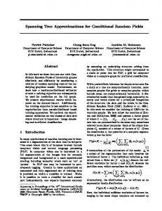
max-margin log-loss ∆ = 1, β = 1 ∆ = 0, β = 3 ∆ = 1, β = 4 1

hw, φ(x, y)i −2

−1

0

1

2

Fig. 1. `β (w, x, y) for different β compared to log-loss and max-margin loss.

the Logistic Regression (LR) classifier. Different instantiations of this loss are visualized in Fig. 1, including the log-loss and the max-margin loss. For the special case of binary classification, the influence of the inverse temperature on `β (x, y, w) was in parts discussed in [6]. In our work we focus on classifiers for structured outputs. In this setting the effective number of negative outputs can be exponentially large, which makes the analysis more complex. 4.3

Regularization by entropy and margin

The dual of our new loss can be found by using the method of Lagrange, resulting in Lemma 2. The derivations are similar as in [7], and the details are in the supplement. Lemma 2. The dual minimization problem corresponding to Equation (2) using our generalized per-example loss `β (w, x, y), is given by N

min u

s.t.

1 XX 1 T u Au − bT u + un,y log un,y 2C β n=1 y∈Y X un,y ≥ 0 and un,y = 1 ∀y, n

(10)

y∈Y

where un,y denotes the dual variable for the output y in training example n and A is given by A(n1 ,y),(n2 ,y0 ) = hgn1 ,y , gn2 ,y0 i. The difference between two mapped outputs is denoted by gn,y = −g(x(n) , y, y (n) ) = φ(x(n) , y (n) )−φ(x(n) , y). Furthermore, all the possible error terms are collected in a vector b: bn,y = ∆(y, y (n) ). A total of N · |Y| dual variables are required. The primal and dual

8

Patrick Pletscher, Cheng Soon Ong, Joachim M. Buhmann

variables are related by w=

N 1 XX un,y gn,y . C n=1 y∈Y

The dual in Equation (10) reveals a double regularization of `β (w, x, y) by a margin term and an entropy term. Unsurprisingly, the log-loss and max-margin loss can also be identified as special cases in the dual: if b is the zero vector, we obtain the dual of the standard CRF, if β → ∞ the dual of the SSVM. 4.4

The effect of the inverse temperature β

So far, we argued that in order to reconstruct the log-loss from `β , the parameters β = 1 as well as a zero error term ∆(y 0 , y) need to be used. However, the dual in Equation (10) shows that it is actually sufficient to only alter the inverse temperature β and the regularization parameter C, but not the error term itself. For a sufficiently small C and β, the error term contribution −bT u becomes negligible compared to the first and third terms. As a result we identify the CRF dual. As we have seen, β changes the sharpness of the conditional probability Pβ (y 0 |y, x, w). For β → 0 all outputs y 0 have an uniform distribution, i.e., Pβ (y 0 |y, x, w) has an entropy of log(|Y|). For β ≈ 1 the distribution behaves as a Gibbs distribution. For large values of β the probability mass concentrates on the outputs with the largest scores. Probabilities on the outputs are in this case not well-defined; the distribution consists of individual, scaled Dirac impulses at the outputs y ∗ with maximum scores. These findings are in line with [8], where SVMs are shown to be incapable of estimating conditional probabilities in a multiclass setting. 4.5

Choosing β

At this point it is natural to ask: “What is the best choice for β?” Ideally, β is optimized based on the training data. However, looking at the dual in Equation (10), a model order selection question arises. By naively minimizing the loss w.r.t. β, this would always result in choosing β → ∞, which is not desired. We thus advocate determining β via cross validation on hold out data.

5

Latent variables

We now turn our attention to structured classifiers for partially observed data. Two training objectives have been suggested for this more challenging setting: The Hidden Conditional Random Field (HCRF) [9], and the Latent Support Vector Machine [10]. Here we show that our formulation also allows for this scenario. Incorporating hidden variables into the output is an important extension of practical relevance: some outputs might for practical reasons be unobservable or one might define a hidden cause that leads to better accuracy of the

Entropy and Margin Maximization for Structured Output Learning

9

predictions. Let us denote the observed variables by y and the hidden, unobserved output variables (latent variables) by z ∈ Z. In HCRFs, the conditional probability of observing y and z are modeled using a Gibbs distribution: Pβ (y, z|x, w) =



 1 exp β w, φ(x, y, z) . Zβ (x, w)

Here, we directly include the inverse temperature β; β = 1 recovers the standard HCRF [9]. The model predicts according to X y ∗ = argmax Pβ (y, z|x, w). y∈Y

z∈Z

Comparing this to the fully observed prediction rule in Equation (1), we see that hidden variables are marginalized out. The introduction of the error terms into the Gibbs distribution by multiplying the two posterior distributions yields Pβ (y 0 , z|y, x, w) =



 1 exp β w∆ , φ∆ (x, y 0 , z, y) . Zβ (y, x, w)

with φ∆ (x, y 0 , z, y) = [φ(x, y 0 , z)T , ∆(y 0 , y)]T . Here it is assumed that ∆(y 0 , y) is only dependent on observed output variables. As in the CRF, training of the parameters is performed by minimizing the regularized negative log-likelihood, scaled by 1/β. However, for the partially observed case, the hidden variables z have to be integrated out. This leads to `β (w, x, y) = −



X  1 log exp β w∆ , φ∆ (x, y, z, y) β z∈Z 

X  1 exp β w∆ , φ∆ (x, y 0 , z 0 , y) . + log β 0 y ∈Y z 0 ∈Z

Taking the limit for β → ∞ and using the log-sum-exp “trick”, the Latent SVM [10] loss emerges:



 `∞ (w, x, y) = − max w∆ , φ∆ (x, y, z, y) + max w∆ , φ∆ (x, y 0 , z 0 , y) . 0 z∈Z

y ∈Y z 0 ∈Z

Again, the Latent SVM can be seen as a probabilistic model, in which all the probability mass is concentrated on the y, z combination with the largest score. The limit case of the inverse temperature also changes the prediction for new test data to y ∗ = argmax hw, φ(x, y, z)i. y∈Y,z∈Z

Instead of marginalizing the hidden variables out, we now maximize them out. The introduction of latent variables in general turns the empirical risk minimization in Equation (2) into a non-convex optimization problem.

10

Patrick Pletscher, Cheng Soon Ong, Joachim M. Buhmann

6

Algorithmic issues

So far we have focused on the theoretical comparison of the different losses for structured output prediction. In this section we will discuss issues that are important for an actual implementation. 6.1

Minimization of the objective

Our new loss `β (w, x, y) is both convex (for the completely observed case) and smooth for any inverse temperature except when β → ∞, thus standard conjugate-gradient or LBFGS solvers are applicable for the minimization of the loss. In our implementations we use the LBFGS solver of minFunc2 . This is contrary to the minimization of the standard max-margin objective, where special algorithms for non-differentiable minimization problems are required. For learning with `β (w, x, y), we are also interested in its derivative w.r.t. w. For fully observed data and margin rescaling, the gradient takes a form similar to that of standard CRFs: X ∂`β (w, x, y) = −φ(x, y) + Pβ (y 0 |y, x, w)φ(x, y 0 ). ∂w 0 y ∈Y

In our implementation we use the gradient information for the efficient minimization of the loss. The LBFGS algorithm computes an approximation to the Hessian of the objective. For small β, this second-order information drastically improves the running time of the training. For large β, the Hessian does not help as the objective becomes essentially piecewise linear. 6.2

Efficient inference in training

One key step in the optimization of the objective function is the evaluation of the log-partition sum Zβ (y, x, w), which is generally computationally intractable. There exist cases, like for example a φ(x, y) that corresponds to a tree structured graphical model, where the computation of Zβ (y, x, w) can be performed efficiently. The SSVM instead requires computing the maximum violating output y ∗ = argmaxy0 ∈Y hw∆ , φ∆ (x, y 0 )i. Both tasks in general are computationally hard, but there exist classes of problems where the maximization is tractable, but not the computation of the partition sum. This is for example the case if submodularity constraints are imposed on the potentials of a general graphical model.

7

Related work

Since [6], there have been various attempts to unify the max-margin and log losses. The connections between SVMs and exponential families have been indicated in [11], and our work makes the link between the log-loss and max-margin 2

http://people.cs.ubc.ca/~schmidtm/Software/minFunc.html

Entropy and Margin Maximization for Structured Output Learning

11

loss more explicit through the inverse temperature and also extends to structured classifiers and latent variables. In [12] an algorithm for learning multiclass SVMs in the primal is discussed: The max-margin loss is approximated by a soft-max, which can then be optimized by a conjugate-gradient solver. [13] considers a loss function similar to ours, applied to multiclass SVM. Two recent papers have appeared which combine the benefits of both the margin idea and the probabilistic model. In [14], a convex combination of log-loss and max-margin loss was proposed. The authors prove Fisher consistency and PACBayes bounds for the resulting classifiers. We conjecture that our model shares many of the advantages of their hybrid model with the additional advantage that it allows for a probabilistic interpretation. Independently, the softmax-margin was developed in [15]. The proposed loss and ours are very similar in spirit: both introduce the margin concept known from SSVMs also into CRFs. In the application of named-entity recognition which they consider, the margin term shows to improve the accuracy of the classifier. However, the connection between CRFs and SSVMs is not established.

8

Experiments

In our experiments we will only consider settings with either a small number of outputs |Y|, or where inference can be performed exactly, such as scenarios where the feature map φ(x, y) corresponds to a chain structured graphical model. 8.1

Multiclass learning

As a first experiment we consider the well-studied multiclass setting in which a data point is assigned to one of K classes. The feature map φ(x, y) as introduced in [16] is used,   δ1 (y)· x  δ2 (y)· x    φ(x, y) =  . ..   . δK (y)· x Here δk (y) denotes the Kronecker Delta function, which is 1 for y = k and 0 everywhere else. For all the multiclass experiments, we report the results of the liblinear3 implementation of LR and SVM as baseline classifiers. Synthetic data We designed three synthetic datasets with the reasoning in Section 4.4 in mind. Each of the datasets shows different characteristics, which can be exploited by the losses. The first dataset, Synth1, consists of three classes. Each class is sampled from a Gaussian with means at 0, 1 and 2 and variance 1. We would expect a small β to perform best on this dataset, as the classes overlap to a large extent. The second dataset, Synth2, consists of three classes. Each 3

http://www.csie.ntu.edu.tw/~cjlin/liblinear/

12

Patrick Pletscher, Cheng Soon Ong, Joachim M. Buhmann Synth2

Synth1

Synth3

test error (%)

44 24.4

43.5

24.2

43

24

42.5

43 42 41 10−1

100 β

101

23.8 0 10

101

102 β

103

42 0 10

101

102

103

β

Fig. 2. Results on the different synthetic multiclass datasets. Changing the parameter β leads to different test errors.

class is sampled from a Gaussian with means at (0, 0), (1, 0.1) and (1, −0.1), each with covariance 0.25I. Here, the prediction error is computed by accounting only 0.1 for a confusion between class 2 and 3, and 1 otherwise. This information is provided to the classifier using the error term. We expect the best results with a large β, as the error term information is crucial. The third dataset, Synth3, consists of four Gaussians. Two of which have means (0, 0) and (1, 0), the remaining two have almost indistinguishable means of (0.5, 0.4) and (0.5, 0.6). All classes have a covariance of I. Again, for the indistinguishable classes we only account an error of 0.1 when confusing them. Here we would expect an intermediate value of β to lead to the best results, as both noise and skewed class importance are present. The training set consists of 2000 examples for each class, the test test of 10000 examples for each class. The test error is averaged over 5 random instantiations of the data set. For all classifiers C = 1 is fixed, as there is enough data to prevent overfitting. The results of this experiment are shown in Table 1 and in Fig. 2. We observe that the inverse temperature can have a substantial influence on the accuracy of the resulting classifier. No value of β is optimal for all three datasets, which is in agreement with the discussion in Section 4.4. The experiment also shows that the limit case of a SVM for β → ∞ is already achieved for a relatively small β. MNIST data We consider the MNIST digits dataset, a real world multiclass dataset. For all experiments a 0/1 error term is used. In a first experiment, we analyze the test error and running time on a random subset of the dataset, where for each digit 100 examples are included. The results are visualized in Fig. 3. We observe that for larger β one needs to increase C in order to get a good prediction error. Furthermore, the running time of the training is substantially smaller for small values of β. In a second experiment we consider the full MNIST data set. Cross validation is performed for determining the regularization parameter C. For the full dataset, contrary to the first experiment where only a subset of the dataset is used, we

Entropy and Margin Maximization for Structured Output Learning

13

Table 1. Synthetic multiclass results. The first row corresponds to a LR, the third row to a SVM. The second row is a specific instance of the novel loss. For the liblinear SVM we use the 0/1 error term (and not the ones described in the synthetic data generation) and thus inferior results are expected for Synth2 and Synth3.

268.4

2

13.5

2

10

10

205.5

loss test error (%) β ∆(y 0 , y) Synth1 Synth2 Synth3 1 no 41.0 ± 0.4 25.8 ± 0.2 43.9 ± 0.2 5 yes 44.0 ± 0.1 24.2 ± 0.1 42.0 ± 0.2 106 yes 44.0 ± 0.1 24.2 ± 0.1 43.7 ± 0.7 liblinear LR 41.7 ± 0.3 26.5 ± 0.2 44.5 ± 0.2 liblinear SVM 44.0 ± 0.1 31.9 ± 0.8 50.2 ± 4.3

14

13.9 1

1

10

79.5

10

β

β

13.1 12.7

13.5

5 2.

0

0

10

10

−1

−1

10

10 4

10

5

10 C

6

10

4

10

5

10 C

6

10

Fig. 3. Contour plot showing the test error (left) and the running time (in seconds) of the training (right) for combinations of β and C on a subset of the MNIST data set.

found the max-margin loss to perform best. Using cross validation the model can automatically determine that a large β is beneficial (second row in Table 2). 8.2

Linear chain model

In this experiment we consider the OCR dataset from [3]. Here, the task is to predict the letters of a word from a given sequence of binary images. By exploiting the dependencies between neighboring letters, the accuracy of the classifier can be improved. We use the same folds as in the original publication: The dataset consists of 10 train/test set splits, with each approximately 600 train and 5500 test sequences. We used the Hamming distance as our error term and perform inference in the linear chain model by libDAI [17]. In our experiments we found, both SSVM and CRF match the test error of around 20% (Fig. 4 right) reported in [3]. Varying the parameter β leads to a small, but consistent improvement over log-loss and max-margin loss (Fig. 4 left). We perform a second experiment on this dataset to evaluate the quality of the probabilities on outputs learned by the model. To do so, we measure

14

Patrick Pletscher, Cheng Soon Ong, Joachim M. Buhmann Table 2. Results on the MNIST dataset for different instantiations of `β .

loss β=1 β = 10 β = 103 liblinear LR liblinear SVM

C test error (%) 105.5 7.5 106 7.1 106 7.1 106 8.4 106 7.1

the error when predicting using the marginal-posterior-mode (MPM) instead of using the MAP predictor. For an individual variable yi of the output y, the MPM marginalizes out all other variables y\yi : X yi∗ = argmax P (y|x, w). yi

y\yi

Using the MPM leads to good accuracy if no error term is included in training, but fails otherwise (Fig. 4 right). This is in agreement with our discussion in Section 4.4 that probabilities on outputs are not well-defined for SSVMs.

test error (%)

error difference (%)

0.4 0.2 0 −0.2 −0.4 −0.6

30 `β CRF

25 20 0

0.1

1

5

β

10

20

50

20

40

60

β

Fig. 4. Results on the OCR dataset. Left: Absolute error difference between the standard CRF and `β . Right: Using MPM prediction when including the error term in training deteriorates the accuracy. The dashed line is the test error of the standard CRF. The solid line corresponds to the test error when training with `β .

8.3

Multiple instance learning

As a last experiment we consider the problem of learning from multiple instances (MIL). This is a scenario with latent variables in training, as the label of an individual instance in a bag is not observed; only the label of the whole bag. The model for β = 1 and no error terms recovers the MI/LR from [18], for β → ∞ the model reduces to the MI-SVM [19].

Entropy and Margin Maximization for Structured Output Learning

15

We construct a one-dimensional synthetic dataset which illustrates the deficiencies of the MI-SVM. A positive bag consists of p positive instances and 50 − p negative (0 < p ≤ 50), a negative bag contains 50 negative instances. The individual instances are hard to classify: the positive instances are Gaussian distributed with mean 0.6 whereas the negative instances are Gaussian distributed with mean 0, the variance for both classes is 1. Smaller values of β lead to better classification performance, as this corresponds to an averaging over the different instances in a bag, which is a good strategy for large data uncertainty (Fig. 5).

test error (%)

50 40

p=1 p = 25

30 20 10−2

10−1

100

101

102

103

104

β Fig. 5. Results for the synthetic MIL dataset for 400 bags, averaged over 10 random data sets. Depending on the number p of positive instances, a small β improves the accuracy substantially. The solid line corresponds to a setting where only one instance per bag is positive, the dashed line to 25 positive instances per bag.

9

Conclusions

We have introduced a novel family of losses for structured output learning. The loss is parametrized by an inverse temperature β, which controls the entropy of the posterior distribution on outputs. The dual of the loss shows a double regularization by a margin and an entropy term. The max-margin loss and the log-loss emerge as two special cases of this loss. Additionally, our work also extends to models with hidden variables. We conjecture that different applications require different values of β and validate this claim experimentally on multiclass, linear-chain models and multiple instance learning. Choosing a large β, which corresponds to a large margin setting, while sometimes improving the accuracy, shows to have the severe disadvantage of deteriorating the probability distribution on outputs. The difference between the losses for different values of β is particularly striking in the multiple instance learning experiment. Acknowledgments We thank Sharon Wulff and Yvonne Moh for proof-reading an early version of this paper. This work was supported in parts by the Swiss National Science Foundation (SNF) under grant number 200021-117946.

Bibliography

[1] J. Lafferty, A. McCallum, and F. Pereira. Conditional random fields: Probabilistic models for segmenting and labeling sequence data. In ICML, 2001. [2] I. Tsochantaridis, T. Hofmann, T. Joachims, and Y. Altun. Support vector machine learning for interdependent and structured output spaces. In ICML, page 104, 2004. [3] B. Taskar, C. Guestrin, and D. Koller. Max-margin Markov networks. In NIPS, 2003. [4] G. Bakir, T. Hofmann, B. Sch¨olkopf, A. Smola, B. Taskar, and S. V. N. Vishwanathan. Predicting Structured Data. The MIT Press, 2007. [5] M. Wainwright and M. Jordan. Graphical models, exponential families, and variational inference. Foundations and Trends in Machine Learning, 2008. [6] T. Zhang and Frank J. Oles. Text categorization based on regularized linear classification methods. Information Retrieval, 4:5–31, 2000. [7] M. Collins, A. Globerson, T. Koo, X. Carreras, and P. L. Bartlett. Exponentiated gradient algorithms for conditional random fields and max-margin Markov networks. J. Mach. Learn. Res., 9:1775–1822, 2008. [8] P. L. Bartlett and A. Tewari. Sparseness vs estimating conditional probabilities: Some asymptotic results. J. Mach. Learn. Res., 8:775–790, 2007. [9] A. Quattoni, S. Wang, L. Morency, M. Collins, and T. Darrell. Hidden-state conditional random fields. PAMI, 29(10):1848–1852, 2007. [10] C. Yu and T. Joachims. Learning structural SVMs with latent variables. In ICML, pages 1169–1176, 2009. [11] S. Canu and A. J. Smola. Kernel methods and the exponential family. Neurocomputing, 69(7-9):714–720, 2006. [12] O. Chapelle and A. Zien. Semi-supervised classification by low density separation. In AISTATS, pages 57–64, 2005. [13] T. Zhang. Class-size independent generalization analysis of some discriminative multi-category classification. In NIPS, Cambridge, MA, 2005. [14] Q. Shi, M. Reid, and T. Caetano. Hybrid model of conditional random field and support vector machine. Workshop at NIPS, 2009. [15] K. Gimpel and N. Smith. Softmax-margin crfs: Training log-linear models with cost functions. In HLT, pages 733–736, 2010. [16] K. Crammer and Y. Singer. On the algorithmic implementation of multiclass kernel-based vector machines. J. Mach. Learn. Res., 2:2001, 2001. [17] J. Mooij. libDAI: A free/open source C++ library for Discrete Approximate Inference, 2009. [18] S. Ray and M. Craven. Supervised versus multiple instance learning: An empirical comparison. In ICML, 2005. [19] S. Andrews, I. Tsochantaridis, and T. Hofmann. Support vector machines for multiple-instance learning. In NIPS, pages 561–568, 2003.