Equalization Based on Particle Filtering for Mobile Station ... - eurasip

15th European Signal Processing Conference (EUSIPCO 2007), Poznan, Poland, September 3-7, 2007, copyright by EURASIP

EQUALIZATION BASED ON PARTICLE FILTERING FOR MOBILE STATION RECEIVERS A. Korah, J. P. Cances, G. Ferré and V. Meghdadi Université de Limoges - Ecole Nationale Supérieure d'Ingénieurs de Limoges (ENSIL) XLIM-Dept. C2S2 UMR CNRS 6172 16, Rue Atlantis - Parc ESTER - BP 6804- 87068 Limoges cedex, France Email {korah,cances,ferré,meghdadi}@ensil.unilim.fr ABSTRACT In this paper, we present the application of particle filtering to build efficient equalizer structures for mobile station terminals. We begin by recalling the theory of particle filtering and we put the emphasis on the key point of such a technique, the sampling importance resampling (SIR) or the sequential importance sampling (SIS). Then, we present a mathematical model which allows to represent the transmitted symbols as the state of a stochastic system which can be estimated by particle filters. Furthermore, we propose a basic equalizer structure with particle filters and we investigate several improvement strategies which help to obtain better estimation results with a lower number of particles. Finally, simulation results in the context of GSM/EDGE are given which show that the proposed particle filter equalizer, outperforms the well known extended Kalman filter. 1.

INTRODUCTION

Particle filters, also known as Sequential Monte Carlo methods (SMC) are sophisticated model estimation techniques based on simulation. They are usually used to estimate Bayesian models and are the sequential analogue of Markov Chain Monte Carlo (MCMC) batch methods. If well designed, particle filters can be much faster than MCMC. They are often an alternative to the Extended Kalman Filter (EKF) with the advantage that, with sufficient samples, they approach the Baeysian optimal estimate. So they can be made more accurate than the EKF. Since the pioneering work of Gordon, Salmond and Smith [1], particle filters are used in many fields. For example image recognition or positioning systems. In the recent years, one can find several papers [2-5] devoted to application to communication systems. In the case of application in baseband algorithms of a mobile station receiver, one can find three main areas of interest for particle filters, symbol estimation, channel estimation and combined, symbol and channel estimation (blind symbol estimation). Blind symbol estimation means to estimate the transmitted symbols without any available channel estimation. This estimation technique, usually applies, when no training data are available to estimate the Channel Impulse Response (CIR) of the wireless link. In fact, blind symbol estimation with particle filters is only suggestive, if no training symbols are used in a communication system. Because of the existence of a Training Sequence Code (TSC) in GSM, we decide not to apply particle filters for blind symbol estimation. Channel estimation algorithms are well investigated for GSM/EDGE. Commonly Least Mean Square (LMS) algorithms are used which obtain good estimation results [6]. For this work, those channel estimation algorithms were applied to estimate the channel. Then, this channel estimation is used as an input parameter for the presented particle filter symbol estimation algorithm.

©2007 EURASIP

The rest of the paper is organized as follows. In section 2 we present the theory of particle filtering by insisting on the SIR or SIS techniques which are fundamental tools in particular filtering. We propose then in section 3 to derive a stochastically model for our communication system which allows to represent the transmitted symbols as the state of a stochastic system which can be estimated by particle filters. In section 4, we detail the structure of our particle filter based equalizer and we discuss about some implementation considerations to improve the performances of the basic structure. Section 5 is devoted to the simulation results including some interesting comparisons with the performances of the EKF structure. Finally, conclusion is given in section 6. 2.

PARTICLE FILTERING THEORY

The particle filter aims to estimate the sequence of hidden parameters xk for k = 0,1, 2..., n , based only on the observed data yk for k = 0,1, 2..., n . All Bayesian estimates of xk follow from the posterior distribution, but rather than the full posterior p ( x0 , x1 , ..., xk y0 , y1 , ..., yk ) , which would be the usual MCMC or importance sampling approach, particle methods estimate the filtering distribution: p ( xk y0 , y1 ,..., yk ) .

Model: Particle methods assume that xk and the observations

yk can be modeled in this form

x0 , x1 ,..., xk is a first order Markov process such that

xk xk −1 ~ p x

k xk −1

( x xk −1 )

and

with

an

initial

distribution p ( x0 ) .

The

observations

y0 , y1 ,..., yk are

conditionally

independent provided that x0 , x1 ,..., xk are known. In other words, each y k only depends on xk . One example form of this scenario can be written in the following way xk = f ( xk −1 ) + vk (1) y k = h ( xk ) + z k where both vk and z k are mutually independent and identically distributed sequences with known probability density functions and f (.) and h (.) are also known functions. These two equations can be viewed as state space equations and look similar to the state space equations for the Kalman filter. If the functions f (.) and h (.) were linear, and if both, vk and

z k were Gaussian, the Kalman filter finds the exact Bayesian

484


filtering distribution. If not, Kalman filter based methods are a first-order approximation. Particle filters are also an approximation, but with enough particles can be much more accurate. Monte Carlo approximation: Particle methods, like all sampling-based approaches (e.g. MCMC) generate a set of samples that approximate the filtering distribution p ( xk y0 , y1 ,..., yk ) . So, with P samples, expectations with respect to the filtering distribution are approximated by 1 P (L) (2) ∫ f ( xk ).p( xk y0 , y1 ,..., yk ).dxk ≈ ∑ f ( xk ) P L =1 and f (.) , in the usual way for Monte Carlo, can give all the moments of the distribution up to some degree of approximation. Generally, the algorithm is repeated iteratively for a specific number of k values (call this N). When done, the mean of xk over all the particles is approximately the actual value of xk .

Sampling Importance Resampling (SIR), is a very commonly used particle filtering algorithm, which approximates the filtering distribution p ( xk y0 , y1 ,..., yk ) by a weighted set of particles

w

( L) k

{(w

( L) k

}

, xk ) : L = 1,..., P . The importance weights ( L)

are approximations to the relative posterior probabilities P

(L)

(or densities) of the particles such that ∑ wk L =1

= 1 . SIR is a

sequential (i.e. recursive) version of importance sampling. As in importance sampling, the expectation of a function f (.) can be approximated as a weighted average. P

∫ f ( xk ) p ( xk y0 , y1 ,..., yk ) .dxk ≈ ∑ w k . f ( xk ) L =1

(L)

(L)

(3)

The algorithm performance is dependent on the choice of the importance distribution, π ( xk x0:k −1 , y0:k ) . The optimal distribution is given as, π ( xk x0:k −1 , y0:k ) = p ( xk xk −1 , yk ) , and

xk( L ) ∼ π ( xk x0:( Lk)−1 , y0:k )

(5)

2-For L = 1,..., P evaluate the importance weights up to a normalizing constant

ˆ (kL ) = w (kL−)1 . w

p( yk xk( L ) ). p( xk( L ) xk( L−1) )

π ( xk x0:( Lk)−1 , y0:k )

(6)

3-For L = 1,..., P compute the normalized importance weights P

ˆ (kL ) ∑ w ˆ (kJ ) w (kL ) = w

(7)

j =1

4-Compute an estimate of the effective number of particles as P Nˆ = 1 ∑ (w ( L ) )2 (8) eff

L =1

k

5-If the effective number of particles is less than a given threshold Nˆ eff < N thr , then perform resampling a) Draw P particles from the current particle set with probabilities proportional to their weights. Replace the current particle set with this new one. b) For L = 1,..., P set w (kL ) = 1/ P . The term Sequential Importance Resampling is also sometimes used when referring to SIR filters. Sequential Importance Sampling (SIS), is the same as SIR, but without the resampling stage. A direct version of the particle filtering algorithm may be implemented in the following way. “Direct version” algorithm-The direct version algorithm is rather simple, it uses composition and rejection. To generate a single sample x at k from px y ( x y1:k ) , k 1:k

1-Set p = 1 2-Uniformly generate L from {1,..., P} 3-Generate a test xˆ from its distribution px

k xk −1

( x xk( L−1) k −1 )

4-Generate the probability of yˆ using xˆ from p y x ( yk xˆ ) where yk is the measured value

is often named importance sampling function. However, the transition prior is often used as importance function, since it is easier to calculate, and also simplifies, the subsequent importance weight calculations π ( xk x0:k −1 , y0:k ) = p ( xk xk −1 ) (4)

5-Generate another uniform u from [0, mk ] 6-Compare u and yˆ a) if u is larger then repeat from step 2 b) if u is smaller then save xˆ as xk k ( p ) and increment p

SIR filters with transition prior as importance function are commonly known as bootstrap filter and condensation algorithm. Resampling is used to avoid the problem of degeneracy of the algorithm, that is, avoiding the situation that all but one importance weights are close to zero. The performance of the algorithm can be also affected by proper choice of resampling method. For example the stratified resampling proposed by Kitagawa [7] is optimal in terms of variance. A single step of sequential importance resampling is as follows 1-For L = 1,..., P draw sample from the importance distributions

7-If p > P then quit The goal is to generate P particles at k, using only the particles from k – 1. This requires that a Markov equation can be written and computed to generate a xk based only upon xk −1 . This algorithm uses composition of the P particles from k – 1 to generate a particle at k and repeats (steps 2→6) until P particles are generated at k. This can be more easily visualized, if x is viewed as a two-dimensional array. Note that, x(k , L)

©2007 EURASIP

would be the Lth particle at k and can also be written xk( L ) (as done above in the algorithm). Step 3 generates a potential xk based on a randomly chosen particle ( xk( L−1) ) at time k – 1 and

485


rejects or accepts it in step 6. In other words, the xk values are generated using the previously generated xk −1 .

3.

MATHEMATICAL MODEL FOR THE COMMUNICATION SYSTEM

For many communication systems (e.g. GSM/EDGE) the mobile radio channel with the effects of multipath propagation and noise, can be described with a Finite Impulse Response (FIR) filter and an additional random variable vk usually assumed to be a sample from a Gaussian distribution. This model can be represented in the following state space form similar to (1).  hk 1   sk      xk = F . xk −1 + bsk  hk 2  ; x =  sk −1  (10) (9), where h = k  ⋮  k  ⋮  yk = hkT xk + vk      hkL   sk − L +1 

0  1 and F = 0  ⋮ 0 

1  0 0 ⋯ 0 0    0 0 ⋯ 0 0 0  1 0 ⋯ 0 0  ; b = 0     ⋮ ⋮ ⋱ ⋮ ⋮ ⋮   0  0 0 ⋯ 1 0  

(11)

The matrix F is used to perform the shifting operation of the input values inside the FIR filter. hkT represents a vector containing the L filter coefficients of the multipath channel FIR model, and xk represents a vector of the L data symbols

[ sk , sk −1 ,..., sk − L +1 ] , transmitted through the channel. Generally, as pointed out by the index k, the vector of the modelled attenuation coefficients hkT is time variant. For the presented application we will consider a quasi static fading channel that is channel parameters remain constant over the duration of one GSM burst but vary from burst to burst. The idea of using particle filters for equalization was to employ them to estimate this state vector xk . For symbol estimation, the desired symbol is then extracted out of the most probable state vector. vk is a complex noise sample from a Gaussian distribution with mean

If the probability density functions of (13) are known, p ( xk yk ) could be calculated for every state xk . However, for practical systems with a discrete state space the effort to do this in real time is too high. For example a typical state space of the channel model for 8PSK modulation in an EDGE receiver has the size of the order of 107 elements (with a typical channel length of 8 with 8 possible values per symbol). Additionally, the equalization problem cannot be solved analytical. That means for exact calculation of the maximum a posteriori probability the required pdf has to be evaluated for every state of the state space. Thus, for practical application p ( xk yk ) is only approximated and this is done by SIR, which is implemented as follows. If the desired pdf p ( xk yk ) would be known, it could be sampled to obtain a set of N so called particles

{ }

Ω = xk

(n)

N

(14) n=1

For N → ∞ it can be shown that [8] 1 N (n) p ( x k yk ) = (15) ∑ δ ( xk − xk ) n = 1 N That means that if a large number of random experiments, according to the probability function p ( xk yk ) can be done, the number of outcomes of xk during these experiments can be used as an approximation of p ( xk yk ) . Practically, this pdf is to be estimated so it cannot be sampled directly. However, as we mentioned in section II, if samples can be generated from a different pdf π ( xk xk −1 , yk ) , which is called importance sampling function, a correct weighting of the particles generated from π ( x ) makes an estimation of p ( xk yk ) possible. This weighting factor is called (as in Section II) importance weight w . ( n)

w

(n) k

∝

p ( xk

π (x

( n) k

x

(n)

yk ) ( n −1) k

, yk )

( n −1)

.w k

(16)

That means an estimation value N

( n) ( n) pˆ ( xk yk ) = ∑ w k .δ ( x k − xk )

zero and variance σ . 2

n =1

(17)

could be calculated. The estimation pˆ ( xk yk ) of the posterior

4.

THE PARTICLE FILTER BASED EQUALIZER

probability function is equal to p ( xk yk ) , if N tends to

p ( xk yk ) can be principally computed according to Bayes theorem

The desired pdf

p ( xk yk ) =

p ( yk xk ). p ( xk xk −1 )

(12) p ( yk ) Because only the maximum probability is to be found for symbol estimation, p ( yk ) can be omitted

p ( xk yk ) ∝ p ( yk x k ). p ( xk xk −1 )

©2007 EURASIP

infinity. The choice of a suitable importance sampling function is of great importance to obtain good performance results of a particle filter. In this paper, we use the prior importance function for the distribution

π ( x ) : π ( xk xk −1 , yk ) = p ( x k

(13)

486

(n)

(n)

x k −1 ) which results in ( n −1)

wk ∝ wk (n)

( n)

. p ( yk xk )

(18)


By using this importance sampling function, only the two probability density function p ( x

(n) k

x

(n) k −1

) and p ( yk x

(n) k

),

have to be known to perform state estimation. The probability p ( xk xk −1 ) can be derived directly from the state transition in the first equation of (9). The function

p ( xk xk −1 ) consists of a deterministic part Fxk −1 and the stochastic part bsk , because the input sk is unknown at the receiver. It is of great use that the sent symbol belongs to a limited known alphabet A . This alphabet consists of two symbols for GSM (GMSK) and eight symbols for EDGE (8PSK). Since we consider uncoded transmissions, symbols of this alphabet are assumed to have the same probability to occur, so this leads to

1  for xk = F . xk −1 + b.sk , sk ∈ A p ( xk xk −1 ) =  A  0 else

(19)

Because the noise is assumed to be sampled from a normal distribution , p ( yk xk ) can be calculated

p ( yk x k ) =

−

1

π .σ

2

yk − hT . xk

2

σ2

.e

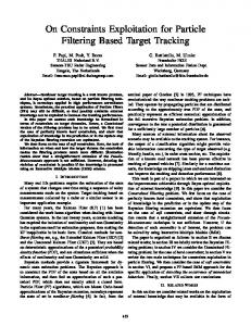
also a high probability. For this reason resampling only duplicates particles with a high probability, and suppresses particles with a low probability. The higher the probability of a particle, the more often a particle is resampled. This method can dramatically improve the performance of the particle filter algorithm. It prevents the algorithm from degeneration [8-9] and it has the additional advantage that the importance weight of a particle from a prior computation step must not be taken into consideration explicitly as in (18). To satisfy the assumption that particles with a high probability for equalization, a prefilter [10] was applied to the channel coefficients to ensure declining coefficients. Implementation concerns - The algorithm shown before for particle filter synthesis is highly parallelizable. It can be implemented in a structure similar as those shown on Fig. 1. Most of the operations applied to a particle can be done independently of other particles. Only the resampling process cannot be implemented that easily in parallel than the other operations. This leads to a very flexible structure for realization in hardware. The SIS part of the algorithm can be done with particle filtering units (PF units) consisting of a particle memory and an operational unit of the SIS algorithm. The number of these units can be defined as a trade-off between area usage and computation speed.

(20)

Using these probability density functions, a new algorithm based on the Direct Version Algorithm, presented in Section II, can be formulated as shown just below. 1-For every time step k do 2-For every particle index n from 1,…,N do ( n)

3-Draw new particle xk

= F . x k -1 + b.sk (n)

( n)

(n)

with sk

uniformly

sampled out of AGMSK or AEDGE / 8 PSK

Figure 1 - Hardware implementation for particle filter equalizer T

ɶ 4-Compute importance weights : w

(n) k

=e

−

yk − h

σ

(n) 2 . xk 2

N

5-Normalize importance weights : w k = wɶ (kn ) ∑ wɶ (km ) (n)

m =1

6-End For 7-Resample particles 8-Select the state xɶ k which occurs most times after resampling as most likely state 9-End For In this algorithm new particles are drawn using the state transition (9). For creating new particles, only values out of the set of valid symbols, AGMSK or AEDGE / 8 PSK , are used. After that the importance weight of the particles is calculated. The steps 2 to 6 are called SIS. For our particular study an additional resampling step was used. In fact, particles in one iteration of the particle filtering algorithm are generated from particles of the iteration before. The assumption, when using resampling, is that particles with a high probability create child particles, with

©2007 EURASIP

For hardware realization, additional improvements of the algorithm can be implemented. In the SIS part of the algorithm the generation of a random symbol sampled from a uniform distribution is needed. Mostly, random numbers are generated with a linear congruential generator [11]. This number is then used as index to select a valid symbol out of a table, which contains the valid symbols according to the used modulation. By simulation, we find that nearly the same performance of the particle filter algorithm can be achieved when using (21), instead of a linear congruential generator, to select a pseudo random symbol out of the table A of the valid symbols according to the used modulation. mn = ( mn −1 + 1) mod( A + 1)

(21)

That means a new table index mn is simply generated by circular counting out of the last table index mn −1 . An other improvement comes from the fact that the variance σ has to be precisely estimated to calculate the importance weight of the

487

2


particles. In the case of the GSM/EDGE system σ is estimated using the training sequence code (TCS) of a GSM burst. Because of its small length of 26 symbols this estimation is not accurate. It was found by simulations, especially at high SNR’s, that the performance of the algorithm could be slightly improved by using already estimated symbols for correction of this noise variance. 2

[5]

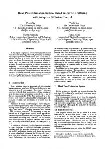
This section shows performance evaluations of the proposed equalization algorithm. For the tested channel we choose a quasi-static frequency selective fading channel with five mean equal power taps in its CIR. That means the CIR contains five taps with mean power 0.2 since we consider normalized power channels. Fig. 2 shows the performance results for GMSK. The simulation was done using different number of particles. In this figure the bit error rate (BER) without any forward error coding (FEC) is shown. The performance was compared to a state of the art reduced state Viterbi algorithm [12]. As an additional performance comparison, the particle filter equalizer was compared to a state of the art estimation algorithm, the Kalman filter. Simulation showed that with comparable computation efforts, particle filters outperform Kalman filter algorithms for symbol estimation as shown in Fig. 3 for 8PSK modulation. As shown in Fig. 2 and Fig. 3 the bit error rate of the particle filter algorithm is scalable by the number of particles used for estimation. For GMSK, satisfying results can be achieved with about 50 particles. For 8PSK approximately 200 particles are needed to obtain good results. So it is supportable that the amount of particles needed for good estimation results also depends on the constellation alphabet size.

[6]

[7]

[8] [9] [10] [11]

[12]

0

10

-1

10

-2

10 BER

SIMULATION RESULTS

6.

[4]

-3

10

CONCLUSION

-4

10

This paper deals with the application of particle filtering to equalization for wireless communication systems over frequency selective fading channels. It was shown that particle filters can outperform some existing performing equalization structures such as the Viterbi equalizer or the Kalman equalizer. However its complexity is much higher than the commonly reduced state Viterbi method. One key point is that, it seems the computational effort for particle filters depends only linearly on the number of channel coefficients of the CIR. This entails that this kind of equalizer could be a promising solution for broadband communication systems with long channel impulse responses. Further works should investigate the feasibility to use the particle filter based equalizer to interface with a channel decoder to obtain a turbo equalizer structure.

Viterbi equalizer PF 50 particles PF 100 particles PF 150 particles

-5

10

0

1

2

3

4 5 SNR (dB)

6

7

8

9

Figure 2 - Simulation results of the particle filter equalizer for GMSK 0

10

-1

10

BER

5.

[3]

Multipath Environment”, EURASIP Journal on Applied Signal Processing, Vol. 2004 (2004), Issue 15, Pages 2306-2314. S. Sénécal, P. O. Amblard, and L. Cavazzana, “Particle Filtering Equalization Method for a Satellite Communication Channel”, EURASIP Journal on Applied Signal Processing, Vol. 2004 (2004), Issue 15, Pages 2315-2327. T. Bertozzi, D Le Ruyet, C Panazio, and H V Thien, “Channel Tracking Using Particle Filtering in Unresolvable Multipath Environments”, EURASIP Journal on Applied Signal Processing, Vol. 2004 (2004), Issue 15, Pages 2328-2338. P. Djuric, J. Kotecha, J. Zhang, Y. Huang, T. Ghirmai, M. Bugallo, J. Minguez, “Particle Filtering”, IEEE Signal Processing Magazine, Vol. 20, pp. 18-38, September 2003. K. Berberidis, T. A. Rontogiannis and S. Thedoridis, “Efficient Block Implementation of the Decision Feedback Equalizer”, IEEE Signal Processing Letter, Vol. 5, n° 6, pp. 129-131, June 1998. G. Kitagawa, “Monte Carlo filter and smoother for non-Gaussian nonlinear state space models”, Journal of Computational and Graphical Statistics, Vol. 5, n° 1, pp. 1-25, 1996. A. Doucet, N. De Freitas, N. Gordon, “Sequential Monte Carlo Methods in Practice”, Springer, New-York, 2001. B. Ristic, S. Arulampalam, N. Gordon, “Beyond the Kalman Filter”, Artech House, Boston 2004. W. H. Gerstacker, R. Schober, “Equalization Concepts for EDGE”, IEEE Trans. on Wireless Comm., Vol. 1, n° 1, pp. 190-199, January 2002. W. H. Press, S. A. Teukolsky, W. T. Vetterling, B. P. Flannery, “Numerical Recipes in C”, Second Edition, Cambridge University Press, Cambridge 1992. J. G. Proakis, “Digital Communications”, McGraw-Hill, New-York, Fourth Edition, 2001.

-2

10

-3

10

REFERENCES [1] N. J. Gordon, D. J. Salmond, A. F. M. Smith, “Novel Approach to non linear / non-Gaussian Bayesian state estimation”, IEEE Proceedings on Radar and Signal Processing, Vol. 140, pp. 107-113, 1993. [2] E. Punskaya, A. Doucet, and W. J. Fitzgerald, “Particle Filtering for Joint Symbol and Code Delay Estimation in DS Spread Spectrum Systems in

©2007 EURASIP

488

Kalman filter equalizer PF 100 particles PF 150 particles PF 200 particles PF 300 particles

-4

10

5

10

15

20

SNR (dB)

Figure 3 - Performance comparison Particle filter/Kalman filter for 8 PSK