communication systems which employ encoders with a higher constraint length ..... S. Haykin, Communication Systems, 4th ed: John Wiley &. Sons Inc., 2000. [2].
ERROR CONTROL CODING BASED ON SUPPORT VECTOR MACHINE Johnny W.H. Kao, Stevan M. Berber Department of Electrical and Computer Engineering, University of Auckland, Auckland, New Zealand ABSTRACT A novel approach of decoding convolutional codes using a multi-class support vector machine is presented in this paper. Support vector machine is a recently developed and well recognized algorithm for constructing maximum margin classifiers. Unlike traditional adaptive learning approaches such as a multi-layer neural network, it is able to converge to a global optimum solution, hence achieving a better performance. However, up to this date so far, no work has yet been done on applying support vector machine on error control coding. In this investigation, decoding is achieved by treating each codeword as a unique class. Hence the decoding procedure becomes a multi-class pattern classification problem. Simulation results show that the bit error rate performance of decoder based on such approach compare favorably with a conventional soft decision Viterbi Algorithm under a noisy channel with additive white Gaussian noise and achieve an extra 2 dB coding gain over the conventional method in a Rayleigh’s fading channel. Index Terms— convolutional codes, Viterbi decoding, support vector machines, pattern classification 1. INTRODUCTION Convolutional code is a widely used class of error control codes that has applications from space satellite communication to digital video broadcasting [1-3]. The Viterbi Algorithm (VA) proposed in 1967 is well known for decoding convolutional code because it is based on maximum likelihood (ML) decoding. However, it is commonly known that the complexity of the VA decoders grows exponentially with the number of constraint length of the encoder, hence makes it less suitable for modern communication systems which employ encoders with a higher constraint length. Moreover, the VA is optimized for memory-less noise, for example an additive Gaussian white noise (AWGN) channel. Therefore for other types of noise impairments in the channel, for example one that experiences Rayleigh’s fading, another procedure of interleaving is commonly introduced, which inevitably increases further latency and complexity in the decoding process [3, 4]. During the past few decades a lot of effort was devoted into finding different alternatives to VA, hoping to
overcome this challenge. Application of methods of artificial intelligence has caught a considerable amount of attention lately because of their ability to solve large scale complex problems. Some examples neural network applications on error control coding and the problem of local minima was revealed by Berber and Wicker in [5, 6]. Support vector machine (SVM), which was first introduced by Vapnik and his co-workers in 1992 becomes immensely successful in the fields of pattern classification and data mining [7-9]. In the recent years, researchers start to recognize the feasibility and the performance of SVMs hence various types of work have been gradually developed to apply such principles in the field of digital communications [10, 11]. In 1995, Dietterich and Bakiri have proposed to solve a multi-class learning problem via error-correcting output codes (ECOC) [12]. Essentially this is using a unique binary codeword to represent one class of object. Thus classification can be realized by solving a series of simpler binary problems within each codeword. Once the codeword is estimated, the unknown object can be identified by maximum likelihood (ML) selection. This method is widely accepted as a way to achieve multi-class learning and studied extensively in [13]. This technique demonstrates that error control coding can be applied since the goal of decoding is to estimate the transmitted codeword and retrieve the original information. However up to this date so far, no literature can be found of applying SVM on error control coding (or channel coding). In this paper therefore, an algorithm of decoding convolutional code using a multi-class pairwise support vector machine is developed and presented. Based on the theory of SVM, a simulator was designed to test the algorithm by comparing its bit error rate (BER) performance to the BER of the conventional VA decoder. 2. SVM DECODER ANALYSIS Conventionally SVM are formulated to classify only two types of objects, or so-called classes. Classification is achieved in two stages: the initial learning or training stage, and the actual decoding stage. At the first stage, some training examples are given to the machine to create certain decision functions in order to differentiate the two classes.
182
During the second stage, the unforeseen object is then classified by those decision rules. To deal with more sophisticated problems, Kreßel introduced a pairwise support vector machine, also known as the one-against-one support vector machine to handle a multi-class problem [14]. In this algorithm, the decision is made from comparing all the combinations of class pairs. Therefore, for a N-class problem, N(N-1)/2 classifiers are constructed. Studies by Hsu [15] and Abe [16] have shown that this algorithm in general is well-suited for a large multiclass problem in terms of performance-complexity tradeoff. Therefore this algorithm is chosen to be applied in the decoder. Consider a set of N message words, m={m1, m2,…, mN,}, where each message word contains k number of binary bits, mi={b1,b2,…,bk}. Each message is associated with a class label, (mi, yi). The message is encoded into an unique codeword xi={x1, x2,…,xt}, which is corrupted by noise after passing through a noisy channel. In another word, the encoder’s task is to map a binary word of k bits long to an encoded word of t bits. Therefore each individual codeword can be regarded as a class with t number of parameters (or features) in each class, where each parameter represents a modulated bit in the codeword.
training data vector xv into the high-dimensional feature space, and bij is a bias term. Define a coefficient vector, wij, such that l ij
w ij = ∑ oqα qφ (x q )
where lij is the number of training data for the ith and jth codeword. To determine the appropriate parameters for wij and bij, the following optimization problem is solved for the training data from comparing the codword i and j [15] l 1 (3) minimize (wij )T wij + C ∑ ξtij 2 t =1 Subject to the following constraints, (wij )T φ(xt ) + b ij ≥ +1 − ξtij , if yt = i
ξtij ≥ 0,C > 0
where C is the tradeoff parameter between the training error ij and the margin of the decision function, and ξt is the slack variable to compensate for any non-linearly separable training points.
m1 ·
ij
d (x) =
∑o
v ij ∈S ij
v ij
αv K (xv , x) + b ij
(4)
(wij )T φ(xt ) + b ij ≤ −1 + ξtij , if yt = j
2.1. Training phase This is an initial stage which only needs to be performed once only, unless the channel condition has varied significantly. The input of the SVM decoder is a set of l number of corrupted sequence that is transmitted from the encoder, which can be represented as (x1, y1), (x2, y2), …, (xl, yl), where xi ∈ ℜt, i = 1,…, l and yi ∈ {1,…, N}. The output is a reduced set of those training data from each codeword pair. These are used as decision variables, also called the support vector (SV). Every SV, denoted by xv, is associated a weighting value αv and a hard decision output ov ∈{+1,-1} to indicate the desired decision result. As this algorithm is comparing two codewords at one time, therefore all combinations of codeword pairs are used during training. Hence this method is also known as one-versus-one SVM. The basic schematic of the training stage is shown in figure 1. During the initial training stage, a decision function for a non-linear SVM is constructed for each combination of codeword pair via,
(2)
q =1
x1 ·
Encoder
·
·
·
·
mN
xN
⊕
SVM Decoder
αv, xv, ov
AWGN
Fig. 1. Overview of the SVM decoder in the training phase.
2.2. Decoding phase At the actual decoding stage, the receiver will observe a noisy sequence, z = {z1,z2,…,zt}. This becomes a new test object for the SVM decoder. The problem of decoding thus becomes a multi-class pattern classification problem. The likelihood of the noisy sequence z is transmitted from the ith codeword can be calculated via,
Di (z) = =
N
∑
j =1, j ≠i N
∑
j =1, j ≠i
ij
sign(d (zij )) S ij
(5)
sign( ∑ α vij ovij K (xvij , z) + b ) ij
v ij =1
ij
for i , j = 1, … , n; j≠i (1) where Sij denotes the set of SVs for the codeword pair ij, K(x,xv)=φT(xv)φ(x) is a kernel function, where φ(x) maps the
This procedure is commonly referred as ‘voting’, and it carries on for i = 1,…,N. Finally the received noisy sequence z is classified to the class label yi which has the highest number of votes. This class label represents the estimate of the transmitted codeword. Once it has been identified, the
183
task of retrieving the associated message mi is not difficult, which is the same as in VA. 2.3. Advantages of SVM decoder The main reason for employing SVM to apply to the decoding problem, over other conventional methods of artificial intelligence, such as a multi-layer neural network, is because there are no local minima problems. Unlike neural networks, SVM is formulated as a quadratic programming (QP) problem. Therefore the global optimum solution, instead of local ones, can be obtained. Moreover, it is more robust to any outliers. In this particular SVM algorithm the training time is reduced because there are less support vectors produced [16]. Like other artificial intelligence systems, the distinct advantage of such algorithm is the adaptability. Through the learning stage, the receiver can have a physical awareness and the ability to adapt to its communication environment, where noise and other types of undesired interferences are impairing the data. Another benefit of an adaptable decoder is that the tradeoff between complexity and error control capability can be controlled according to the application. For traditional error control algorithms, the decoding procedures are usually fixed, regardless to the quality of the channel. Therefore the bit error rate may exceed to the user’s requirement, especially when the signal-to-noise ratio (SNR) is increased. This may imply that some extra time and energy is wasted for the performance that the user does not need. In support vector machines, both the accuracy and the complexity of the decoder are governed by the number of the support vectors produced during the training stage, which are relatively under the designer’s control. Therefore this algorithm has great potentials for the emerging softwaredefined radios where adaptability becomes the essential consideration. 2.4. Complexity of SVM decoder Currently the main assumption in employing such a technique is that the number of possible messages N must be finite so the receiver can create the decision rules for all the possible outcomes. If N gets greater, more decision functions need to be constructed hence the decoding complexity is increased. This could be considered as one of possible constraints in application of this method. The analysis of complexity of SVM is completely different for the two phases. The complexity of SVM during the training phase is related to the optimization algorithm that it is used to solve the QP problem [10]. At the testing phase, where all the support vectors have been identified, the complexity will be the same, regardless of the training algorithm. For the application of error control coding, it mainly concerns with the computational complexity at the
testing stage because the training stage only constitutes a very insignificant amount of time comparing to the total decoding time. Table 1 compares the computational complexity of SVM at the decoding stage with other conventional methods for decoding convolutional code, such as the soft-output Viterbi Algorithm (SOVA) and the maximum a posteriori (MAP) algorithm. The complexity of SVM is derived from examining the number of operators required for a complete classification, which is based on equation (5). The conventional methods are taken from the study in [3]. The comparison is made on these two algorithms because they are currently the two most popular decoding algorithms for convolutional codes [3]. Also, the current SVM decoder uses a radial basis function (RBF) kernel, which requires exponential operations, similar to the conventional MAP algorithm. It is interesting to observe from table 1 that the complexity of SVM decoder has a vastly different characteristic comparing to conventional methods. It is completely controlled by the number of support vectors and the length of codeword to be processed, whereas the conventional algorithms depend heavily on the structure of the encoder. Therefore, as the number of memory elements increases in the encoder, the decoding complexity for SOVA and MAP must increase exponentially as shown from table 1. This is a major drawback of those techniques for applications such as deep space communication where the order of memory can reach to 10 [17]. However, this would not have any effect for the SVM decoder as long as the length of each codeword remains the same. The independency of encoder structure becomes another advantage for the SVM decoder. Although the SVM decoder can only process t bits at a time, multiple decoders can be employed in parallel to increase the decoding speed. 3. DESIGN OF SVM DECODER A simulator of a communication system that consists of a rate 1/2 convolutional encoder, AWGN channel and a pairwise-SVM decoder are designed in order to evaluate the BER performance of SVM decoder. The convolutional encoder can be defined with the octal form of G=4/5. Figure 2 shows the structure of the rate 1/2 convolutional encoder used.
Fig. 2. The rate 1/2 convolutional encoder used in the simulator.
184
TABLE I COMPUTATIONAL COMPLEXITY OF SVM AND OTHER DECODING ALGORITHMS.
# Multiplications
SVM*
SOVA**
MAP**
N (N − 1) (s(t + 2)) 2
T ⎡⎣2 (2k ⋅ 2v )⎤⎦
T ( 5 ⋅ 2k ⋅ 2v + 6 )
-
-
T ⎡⎣2 ( 2 ⋅ 2k ⋅ 2v + 9 ) ⎤⎦
T ( 2 ⋅ 2k ⋅ 2v + 6 )
-
T ( 2 ⋅ 2k ⋅ 2v )
N (N − 1) (st ) 2 N (N − 1) (st + s ) 2 N (N − 1) (s ) 2
# Subtractions # Additions # Exponentials
* A RBF kernel function is assumed; t is the length of the whole codeword to classify; N is the total number of possible codewords; s is the number of support vector in each class. ** k and v is the number of input and the memory elements of the encoder respectively; T is the number of time stages required to decode the same amount of information as the SVM decoder. A readily available software called LIBSVM [18], is implemented for constructing the pairwise SVM and for training and testing the data points. The radial basis function (RBF) is chosen as the kernel function to map the input space to the higher dimensional feature space. The RBF function with a width of γ is defined as, 2
K (x, y) = exp(−γ x − y )
(6)
where the value of γ is set at the recommended value of 1/N. According to [19], the performance of RBF kernel is much comparable to other types of kernel, such as a polynomial or linear function. Hence at this stage there is no need to consider those other kernels. To produce the training data, all the possible codewords from a message of certain length, were corrupted by additive Gaussian noise at SNR of 0 dB and sent repeatedly to the pairwise SVM decoder to generate the decision functions. It was deliberately set at a high noise level to represent the ‘worst-case’ scenario. Then at the testing stage, monte carlo simulations were conducted of random codeword and tested in various levels of noises. The received signal was classified by the pairwise SVM decoder and hence the original message word can be estimated directly because of the one to one correspondence between the message and code word is assumed. This cycle is repeated while recording the number of errors that the decoder makes.
Message Source
Conv. Encoder
BPSK Modulator
SVM Decoder
BPSK Demodulator
Fig. 3. Schematic blocks of the simulating system.
4. SIMULATION RESULTS AND DISCUSSION 4.1. Effect of training size The initial simulation investigates the impact of using different number of training data on the decoding accuracy. There are a total of 16 possible codewords to classify at the decoder’s side. For simulation purposes, the length of codeword to be processed at one time is 8 bits. The channel consists of additive Gaussian noise with a zero mean and variance (i.e. noise power) of N0/2. Table 2 summarizes the results of the SVM decoder. TABLE II SVM PERFORMANCE UNDER DIFFERENT TRAINING SIZES BER Training Training #SVs (SNR 0 dB) Size time (s)* 160 0.0625 153 0.012 480 0.0938 372 0.008 1,600 0.2344 879 0.006 * Simulations were conducted on an Intel Pentium 4 computer with a CPU of 2.4 GHz running Matlab®.
AWGN Channel Data Sink
In all simulations, simple binary phase shift keying (BPSK) was used for modulation. In addition, a well-known soft-decision Viterbi decoder, which is a conventional convolutional decoder, was implemented in the simulator as a benchmark to compare the bit error rate (BER). Figure 3 shows the schematic of the simulated system.
Figure 4 shows the BER curve obtained by the SVM decoder in comparison with the traditional Viterbi decoder, which is based on maximum likelihood (ML). The results are comparable with the Viterbi decoder if adequate training data is given, suggesting that SVM does tend to converge to a global optimum solution (similar to ML decoding). The
185
small training time, shown from table 2, is an advantage of using a pairwise algorithm. Moreover, with a higher training size hence a larger number of support vectors (decision variables), the BER results are generally better as expected. However, there is a limit that the training data can improve the decoder’s performance. Beyond that, not only the decoding accuracy is saturated, also the decoding time will be extended if more support vectors are generated from the trained model. Figure 5 displays the result of such investigation, showing that the performance gain is generally saturated when the number of training data reaches over 1000. −1
10
4.2. Effect of codeword size The number of classifiers will increase exponentially as the number of codewords increases, which is due to a longer message size. This also implies a much longer processing time. This problem, also known as the curse of dimensionality, is one of the drawbacks of pairwise SVM. Figure 6 shows that a longer code sequence in general performs slightly better than a shorter code. This is possibly due to more input features for the SVM decoder to classify or a higher hamming distance to separate each codeword. Nevertheless the trade-off is the long decoding time. This would possibly limit the size of the codeword to be processed at one time. More investigations are undertaken to overcome this difficulty.
−2
10
−3
10
No Coding SVM − training size = 160 SVM − training size = 480 SVM − training size = 1600 Viterbi
−4
10
0
1
2 E /N (dB) s
BER
BER
−2
10
−3
10
No coding Viterbi SVM, msg size = 4 SVM, msg size = 8
−4
3
10
4
o
Fig. 4. BER of the SVM decoder for each different training sizes. 0
−2
BER −3
10
1500 2000 Training Size
2500
3 4 Es/No (dB)
5
6
4.3. Effect of Rayleigh’s fading
10
1000
2
Fig. 6. BER of the SVM decoder for different number of codewords to classify; training size is 1600.
No coding Viterbi SVM
500
1
3000
Fig. 5. BER of the SVM decoder under different training sizes; Es/No fixed at 2 dB.
To further explore the BER characteristic and the system performance of the SVM decoder, the AWGN channel in the simulator is replaced with a Rayleigh fading channel. It is a popular model for estimating the fading characteristics in a land mobile radio channel [1]. In the simulation, no interleaver was used as a compensation for the bursting errors in the fading channel. Figure 7 demonstrated a coding gain of 2 dB from the SVM decoder over the conventional Viterbi decoder. Such improvement is due to the adaptive nature of this decoding scheme, which makes it suitable for more erratic channel conditions. In this example, the Viterbi algorithm is optimized for Gaussian, memory-less channel, therefore it is less effective for a fading channel, in which the noise and the fading signal have a memory-like behavior.
186
[6] −1
10
BER
[7]
[8]
−2
10
No Coding
[9]
Viterbi −3
SVM
10
−2
[10]
0
2 4 E /N (dB) s
6
8
o
Fig. 7. BER of the SVM decoder under Rayleigh’s fading; training size is 1600.
[11] [12]
5. CONCLUSIONS This paper presents a completely new approach to decode convolutional code using support vector machines. By treating each codeword as a unique class, classification can be realized by a pairwise SVM. Simulation results suggest that the BER of the SVM decoder is comparable and even better than the conventional Viterbi Algorithm for the simulated cases; and a coding gain of 2dB is achieved under a Rayleigh’s fading channel. However, the number of codewords to identify is currently a limiting factor for the decoder, which can be compensated by parallel processing. Nevertheless, the independency of encoder structure and adaptability to channel conditions makes this decoder scheme stand out from other conventional decoders.
[13]
ACKNOWLEDGEMENT
[19]
[14] [15]
[16] [17] [18]
The authors would like to thank Assoc. Professor Vojislav Kecman from the University of Auckland for his helpful advice on this research project. REFERENCES [1] [2]
[3] [4]
[5]
S. Haykin, Communication Systems, 4th ed: John Wiley & Sons Inc., 2000. W. C. Huffman and V. Pless, Fundamentals of ErrorCorrecting Codes. Cambridge: Cambridge University Press, 2003. V. Branka and J. Yuan, Turbo Codes- Principles and Applications, 3rd ed: Kluwer Academic, 2002. B. Bougard, A. Giulietti, and L. Van der Perre, Turbo Codes-Desirable and Designable. New York: Kluwer Academic Publisher, 2004. S. M. Berber, P. J. Secker, and Z. A. Salcic, "Theory and application of neural networks for 1/n rate convolutional decoders," Engineering Applications of Artificial Intelligence, vol. 18, pp. 931-949, 2005.
187
X.-A. Wang and S. B. Wicker, "An artificial neural net Viterbi decoder," Communications, IEEE Transactions on, vol. 44, pp. 165-171, 1996. E. Brorvikov, "An Evaluation of Support Vector Machines as a Pattern Recognition Tool," University of Maryland, College Park 1999. K. K. Chin, "Support Vector Machines applied to Speech Classification," in Department of Computer Speech and Language Processing, Master of Philosophy Thesis. Cambridge: University of Cambridge, 1999. L. Wang, Support Vector Machines: Theory and Applications. Berlin: Springer, 2005. T.-M. Huang, V. Kecman, and I. Kopriva, Kernal Based Algorithms for Mining Huge Data Sets. Berlin: Springer, 2006. L. Wang, Soft Computing in Communications. Berlin: Springer, 2004. T. G. Dietterich and G. Bakiri, "Solving Multiclass Learning Problem via Error-Correcting Output Codes," Journal of Artificial Intelligence Research, vol. 2, pp. 263286, 1995. A. Passerini, M. Pontil, and P. Frasconi, "New Results on Error Correcting Output Codes of Kernel Machines," IEEE Transactions on Neural Networks, vol. 15, pp. 45-54, 2004. U. Kreßel, Pairwise classification and support vector machines. Cambridge, MA: MIT Press, 1999. C.-W. Hsu and C.-J. Lin, "A comparison of methods for multiclass support vector machines," Neural Networks, IEEE Transactions on, vol. 13, pp. 415-425, 2002. S. Abe, Support Vector Machines for Pattern Classification. London: Springer, 2005. R. Wells, Applied Coding and Information Theory for Engineers. New Jersey: Prentice-Hall Inc., 1999. C.-C. Chang and C.-J. Lin, "LIBSVM - A Library for Support Vector Machines," 2.82 ed, 2001. Software available at http://www.csie.ntu.edu.tw/~cjlin/libsvm. S. Keerrthi and C.-J. Lin, "Asymptotic behaviors of support vector machines with Gaussian kernel," Neural Computation, vol. 15, pp. 1667-1689, 2003.