10218
JOURNAL OF CLIMATE
VOLUME 26
Error Covariance Estimation for Coupled Data Assimilation Using a Lorenz Atmosphere and a Simple Pycnocline Ocean Model GUIJUN HAN AND XINRONG WU Key Laboratory of Marine Environmental Information Technology, State Oceanic Administration, National Marine Data and Information Service, Tianjin, China
SHAOQING ZHANG NOAA/GFDL, Princeton University, Princeton, New Jersey
ZHENGYU LIU Center for Climate Research and Department of Atmospheric and Oceanic Sciences, University of Wisconsin–Madison, Madison, Wisconsin, and Laboratory of Ocean-Atmosphere Studies, Peking University, Beijing, China
WEI LI Key Laboratory of Marine Environmental Information Technology, State Oceanic Administration, National Marine Data and Information Service, Tianjin, China (Manuscript received 18 April 2013, in final form 17 July 2013) ABSTRACT Coupled data assimilation uses a coupled model consisting of multiple time-scale media to extract information from observations that are available in one or more media. Because of the instantaneous exchanges of information among the coupled media, coupled data assimilation is expected to produce self-consistent and physically balanced coupled state estimates and optimal initialization for coupled model predictions. It is also expected that applying coupling error covariance between two media into observational adjustments in these media can provide direct observational impacts crossing the media and thereby improve the assimilation quality. However, because of the different time scales of variability in different media, accurately evaluating the error covariance between two variables residing in different media is usually very difficult. Using an ensemble filter together with a simple coupled model consisting of a Lorenz atmosphere and a pycnocline ocean model, which characterizes the interaction of multiple time-scale media in the climate system, the impact of the accuracy of coupling error covariance on the quality of coupled data assimilation is studied. Results show that it requires a large ensemble size to improve the assimilation quality by applying coupling error covariance in an ensemble coupled data assimilation system, and the poorly estimated coupling error covariance may otherwise degrade the assimilation quality. It is also found that a fast-varying medium has more difficulty being improved using observations in slow-varying media by applying coupling error covariance because the linear regression from the observational increment in slow-varying media has difficulty representing the high-frequency information of the fast-varying medium.
1. Introduction Given the importance of the balance and coherence of different model components (or media) in coupled model initialization, it has been realized that for the purpose of
Corresponding author address: Guijun Han, National Marine Data and Information Service, 93 Liuwei Road, Hedong District, Tianjin 300171, China. E-mail:
[email protected] DOI: 10.1175/JCLI-D-13-00236.1 Ó 2013 American Meteorological Society
climate estimation and model initialization, data assimilation should be performed within a coupled model framework (e.g., Chen et al. 1995; Zhang et al. 2007; Chen 2010). When the observed data in one or more media are assimilated into the model, information is exchanged among different media in the coupled system. Such an assimilation procedure is called coupled data assimilation (CDA). CDA is expected to produce self-consistent coupled state estimates and optimal initialization for coupled model predictions (e.g., Zhang et al. 2007; Singleton 2011).
15 DECEMBER 2013
10219
HAN ET AL.
In a CDA system, there exists two ways through which observed information in a medium can be transferred to the other media. One way is through fluxes between two coupled media, which is built in by coupled dynamics. Coupled dynamics transfer information between coupled media in a dynamically consistent way, but observational signals may be distorted by the imperfect model. The second way is to directly project observed information in one medium to another by coupling error covariance. Although coupling error covariance also uses the imperfect model information, the observational signals can be transferred to other media instantaneously. A coupling error covariance measures the covarying strength of two variables residing in different coupled media and thus is a key to project observed information from one medium to another. However, the time scales at which the flows vary in different media are different; therefore, it is difficult to accurately evaluate a coupling error covariance between two variables in different media. Apparently, if the evaluated coupling error covariance is not accurate enough, the direct observational adjustment resulting from the coupling error covariance may not improve the assimilation quality. How to use coupling error covariance to enhance observational constraints in CDA is an important and urgent research topic. In this study, we employ an ensemble filter (e.g., Evensen 1994; Whitaker and Hamill 2002; Anderson 2001, 2003) that consists of a simple coupled model and the ensemble adjustment Kalman filter (EAKF; Anderson 2001) to examine the impact of the accuracy of the evaluated coupling error covariance on the quality of CDA. The simple coupled model includes a fast atmosphere and slow upper ocean coupled to a much slower deep ocean as well as an idealized sea ice component. Although the simple coupled model does not have complex physics as a coupled general circulation model (CGCM), it does characterize the interaction of multiple time-scale media in the climate system (Zhang et al. 2013). The simple model can help us clearly understand the essence of the problem we want to address here. This paper is organized as follows. Section 2 briefly describes the simple coupled model and the ensemble filter. The impacts of coupling error covariance on the quality of CDA and climate prediction skill are investigated in sections 3 and 4, respectively. Conclusions and discussion are given in section 5.
2. Methodology a. Brief description of a simple atmosphere–ocean– ice coupled model To clearly address the fundamental issues in the use of coupling error covariance for ensemble CDA raised in
section 1, we employ a simple coupled model that consists of Lorenz’s chaotic atmosphere model (Lorenz 1963), the variations of upper-ocean and pycnocline depth (Zhang 2011a,b; Zhang et al. 2012), and a simple sea ice model (Zhang et al. 2013). The governing equations are x_ 1 5 2sx1 1 sx2 x_ 2 5 2x1 x3 1 (1 1 c1 w)kx1 2 x2 x_ 3 5 x1 x2 2 bx3 Om
w_ 5 c2 x2 1 c3 h 1 c5 wh 2 Od w 1 Sm 1 Ss cos(2pt/Spd ) 2 c7 ut21
G
h_ 5 c4 w 1 c6 wh 2 Od h ut 5 F(x2 , w, ut21 ) ,
(1)
where the six model variables represent the atmosphere, the ocean, and the sea ice [x1, x2, and x3 are for the atmosphere (hereafter denoted by x1,2,3 if present together), w is for the slab ocean, h is for the deep-ocean pycnocline, and u is for the sea ice concentration]. A dot above the variable denotes the time tendency. For the Lorenz atmosphere, the original parameters of s, k, and b with their standard values of 9.95, 28, and 8/3 sustain the chaotic nature of the atmosphere, while c1 represents the oceanic forcing on the atmosphere. For the equation of w, Om is the heat capacity of the ocean and c2 represents the atmospheric forcing on the ocean. The parameters c3 and c5 denote the linear forcing of the deep ocean and the nonlinear interaction of the upper and deep oceans. The term Od denotes the damping coefficient of the slab ocean variable w. The parameters Sm and Ss define the magnitudes of the annual mean and seasonal cycle of the forcings. The term Spd is chosen as 10 so that the period of the forcing is comparable with the oceanic time scale, defining the time scale of the model seasonal cycle. The parameter c7 is the coupling coefficient from the sea ice to the slab ocean. For the pycnocline model, h represents the anomaly of ocean pycnocline depth, and its tendency equation is derived from the two-term balance model of the zonal–time mean pycnocline (Gnanadesikan 1999). The G is a constant of proportionality, while c4 and c6 represent the linear forcing of the upper ocean and the nonlinear interaction of the upper and deep oceans. Finally, the sea ice model is a simple nonlinear function that transfers an enthalpy space to the sea ice concentration space. While the details of the idealized sea ice model can be found in Zhang et al. (2013), here we briefly describe it as follows. To solve the assimilation issue caused by the discontinuous distribution of sea ice concentration (Zhang et al. 2013), the enthalpy (H 5 c8x22 1 c9w2 1 c10ut21)— an extremely simplified nonlinear function of x2, w, and
10220
JOURNAL OF CLIMATE
VOLUME 26
FIG. 1. Time series of (a) x2, (b) w, (c) h, and (d) H with 0, 1, 0, 0, 0, and 0 as the initial conditions for x1, x2, x3, w, h, and u. Note that the shown time periods of x2, w, h, and H are set to 25, 250, 2500, and 50 TUs, respectively, in order to better visualize their variations.
u—is introduced to define the sea ice medium. The nonlinear transformation function from the enthalpy to ice concentration is u 5 F(H) 8 0, H . Hig > > < H , Him 5 1, , > > 21 : 2 ( H 2H )/ H ig 0 ], H 0:5[e2(H2Him) 1 e im # H # Hig (2) where Hig and Him represent the enthalpy thresholds at the point of ice genesis and ice maintenance, respectively, and H0 is a coefficient to adjust the shape of the curve between 0 and 1. The model is set with the parameter values of (s, k, b, c1, c2, c3, c4, c5, c6, c7, c8, c9, c10, Om, Od, Sm, Ss, Spd, G, g, Hig, Him, and H0) 5 (9.95, 28, 8/3, 0.1, 1, 0.01, 1, 0.01, 0.01, 0.1, 0.1, 10, 10, 10, 1, 10, 1, 10, 100, 0.25, 50, 10, and 80). By using a leapfrog time differencing scheme (Dt 5 0.01) with a Robert–Asselin time filter (Robert 1969; Asselin 1972), where the time filtering coefficient is set as g 5 0.25 and starting from the initial conditions
(x1, x2, x3, w, h, and u) 5 (0, 1, 0, 0, 0, and 0), the model is first spun up for 104 nondimensional time units (TUs; 1 TU 5 100 time steps). Figure 1 shows the time series of x2, w, h, and H [note that the time axis is set to reflect the different time scale for each variable and obviously that x2 (h) has the shortest (longest) time scale]. According to the formula of H, it has time scales of both x2 and w. Such a simple model system that has multiple time scales can facilitate our investigation of the use of coupling error covariance cross multiple media that have different time scales.
b. Ensemble coupled data assimilation In this study, we employ a derivative of the sequential ensemble Kalman filter EAKF (Anderson 2001) to implement the coupling error covariance adjustment. The assumption of independence of observational error allows EAKF to sequentially assimilate observations. While the sequential implementation provides much computational convenience for data assimilation, the EAKF maintains the nonlinearity of background flows as much as possible (Anderson 2003; Zhang and Anderson 2003). For the kth observation, denoted as yk, the EAKF
15 DECEMBER 2013
10221
HAN ET AL.
TABLE 1. Observations and adjusted state variables in different data assimilation schemes for SVA, SMA, and MMA, where the superscript ‘‘obs’’ represents the observation while variables without the superscript indicate states to be adjusted.
SVA SMA MMA
xobs 1
xobs 2
xobs 3
wobs
Hobs
x1 x1, x2, and x3 x1, x2, x3, w, and H
x2 x1, x2, and x3 x1, x2, x3, w, and H
x3 x1, x2, and x3 x1, x2, x3, w, and H
w w x1, x2, x3, w, h, and H
H H x1, x2, x3, w, and H
consists of the following two steps: the first step computes the observational increment [see Eqs. (2)–(5) in Zhang et al. (2007)], and the second step projects the observational increment onto related model variables using a uniform linear regression formula: Dxk,i 5
cov(x, yk ) Dyk,i , s2k
(3)
where Dyk,i represents the observational increment of yk for the ith ensemble member. The term Dxk,i is the contribution of the kth observation to the model variable x for the ith ensemble member. Here, cov(x, yk) denotes the error covariance between the prior ensemble of x and the model-estimated ensemble of yk. The parameter sk is the standard deviation of the modelestimated ensemble of yk. If x and y are from different media, then x–y coupling error covariance is involved.
c. Biased twin experiment setup To imitate the real world scenario with various model biases, we design a biased twin experiment that assumes the parameter error is the only source of model biases. The coupled model with the standard parameter values produces the true solution and observations. After the model is spun up for 104 TUs, starting from the initial condition given in section 2a, observations are produced by adding a Gaussian white noise to the true values of x1,2,3, w, and u at the intervals of 5 time steps for x1,2,3 and 20 time steps for w and u. These observational frequencies simulate the feature of the real climate observing system in which the atmospheric observations are available more frequently than the ocean and sea ice. According to the governing equation of w, the seasonal cycle is defined by 10 TUs, and therefore a model year (decade) is 10 (100) TUs. Also, to simulate the lack of deep-ocean measurements in the real observing system, no observation is available for h. The standard deviations of observational errors are 2 for x1,2,3, 0.5 for w, and 0.1 for u. When the sea ice observations are available, the observations of H are calculated according to the definition of H, by using the observations of x2, w, and u. The assimilation model in which all physical parameters of s, k, b, c1, c2, c3, c4, c5, c6, c7, c8, c9, c10, Om, Od, Sm, Ss, Spd, G, and g are set to be 1% greater than their
standard values is used in the assimilation experiments. A Gaussian white noise with the same standard deviations as the observational errors is added on the model state at the end of spinup to form the ensemble initial conditions from which the ensemble filtering data assimilation starts. The total data assimilation period is 10 000 TUs with the first 1000 TUs being the spinup of data assimilation. All statistics are computed using the results of the last 9000 TUs. A two time level adjustment scheme (Zhang et al. 2004), that is the observations at time t are allowed to adjust states at time t 2 1 and t simultaneously, is employed in all data assimilation experiments in this study. Note that, throughout this study, we use coupling error covariance to define the error covariance of two variables residing in different media while using ‘‘cross error covariance’’ to represent the error covariance between two variables residing in the same medium. The analysis is based on the verification of four experiments: 1) model control run (CTL) with no observational constraint; 2) single variable assimilation (SVA), in which the observations of a model variable are only allowed to impact this variable itself ; 3) single medium assimilation (SMA), in which multivariate assimilation is performed in each medium through the use of cross error covariance within the medium; and 4) multiple media assimilation (MMA), in which the coupling error covariance is used to assimilate one medium’s observations into the other media. Table 1 lists the details of the three schemes of SVA, SMA, and MMA, where the superscript ‘‘obs’’ represents observations and Hobs is the observation of enthalpy that is computed with the observations of x2, w, and u. Although a nonlinear relationship exists between H and x2, w, and u, we still simply set the standard deviation of observational errors of H as 3, without changing the essence of the problem we are addressing. In SVA, observations of x1, x2, x3, w, and H are only allowed to adjust themselves. Based on SVA, observations of x1, x2, and x3 in SMA are further allowed to adjust (x2, x3), (x1, x3), and (x1, x2), respectively. Based on SMA, observations of x1, x2, x3, w, and H in MMA are further allowed to adjust (w, H), (w, H), (w, H), (x1, x2, x3, h, H), and (x1, x2, x3, w), respectively. Thus, the difference between SMA and MMA is the use of only cross error covariance for SMA and both cross
10222
JOURNAL OF CLIMATE
and coupling error covariances for MMA in the filtering equation [Eq. (3)]. From the view of the Kalman gain, SVA constrains the Kalman gain matrix to be diagonal, and SMA constrains the cross covariances between media to vanish, and MMA uses the full ensemble Kalman filter. It should also be noted that SVA, SMA, and MMA use the same observations. To examine the impact of ensemble size on the quality of the evaluated coupling error covariance, we perform an array of experiments with different ensemble size (20, 50, 100, and 200) for all three data assimilation schemes. Since the coupling error covariance may require a large ensemble size to reach a high quality, we also examine some large ensemble sizes (e.g., 500, 1000, 2000, 5000, 10 000, and 15 000). Although many sophisticated algorithms of the inflation scheme (e.g., Anderson 2007, 2009; Li et al. 2009; Miyoshi 2011) exist for the filtering in an atmosphere model, the filtering inflation for a coupled model is a new subject due to the multiple time-scale nature of the system (more discussions on this issue will be given in section 3b). Furthermore, trial-and-error experiments show that the usual forms of inflation (e.g., only applying inflation to the atmosphere or equally inflating ensemble spreads of all variables) lead the analysis to increase to infinity, so the numerical calculation halts because of the overflow. Thus, for simplicity and convenience of comparison, in this study, we do not use any inflation for any of our assimilation experiments.
3. Impact of coupling error covariance on ensemble coupled data assimilation a. Sensitivity of the coupling error covariance with respect to ensemble size We first examine the performances of SVA, SMA, and MMA with a default ensemble size (20) that has been used in previous studies (e.g., Zhang and Anderson 2003; Zhang 2011a,b; Liu et al. 2013). Figure 2 shows the root-mean-square errors (RMSEs) of x1,2,3, w, h, and H for SVA, SMA, and MMA with this small ensemble size, where the RMSE of x1,2,3 is the arithmetical average of the RMSEs of x1, x2, and x3. Here, the RMSE used is defined by sffiffiffiffiffiffiffiffiffiffiffiffiffiffiffiffiffiffiffiffiffiffiffiffiffiffiffiffiffiffiffi 1 N RMSE 5 å (z 2 zti )2 , N i51 i
(4)
where N represents the number of analysis steps during the last 9000 TUs for the state variable z that is a unified notation of x1, x2, x3, w, h, and H, and z and zt are the ensemble mean and the truth of z, respectively.
VOLUME 26
FIG. 2. The RMSEs of x1,2,3, w, h, and H for SVA, SMA, and MMA with an ensemble size of 20. Note that all the RMSEs have been normalized by the values of CTL, and the RMSE of x1,2,3 is the arithmetical average of the RMSEs of x1, x2, and x3.
Note that the RMSEs in Fig. 2 have been normalized by the corresponding values for CTL (14.4 for x1,2,3, 1.66 for w, 0.86 for h, and 66.94 for H) that are also computed according to Eq. (4). It clearly shows that SVA behaves best while MMA performs worst. To look into the details, we show the time series of RMSEs1 of x2, w, h, and H (see Fig. 3). Note that since both the truth and CTL are spun up, then the variability of the RMSE of CTL is just the RMS difference of two randomly selected trajectories from the two runs (i.e., there is no initial condition information or observational constraint in the time evolution). SVA maintains a small and nearly stationary error for all model variables, while SMA introduces large oscillations into high-frequency variables (x1,2,3 and H) with the use of cross error covariances among x1, x2, and x3. Compared to SMA, the coupling error covariances make MMA even more unstable for all variables whose errors are almost comparable to that of CTL. Therefore, for a small ensemble size, the
1 Note that the RMSE in Figs. 3–6 and 9 is different from that in Figs. 2, 7, and 10 that use Eq. (4). At a given analysis step the qffiffiffiffiffiffiffiffiffiffiffiffiffiffiffiffiffiffiffiffiffiffiffiffiffiffiffiffiffiffiffiffiffiffi K RMSE is normally defined as åi51 (zi 2 zti )2 /K, where K represents the number of state variables or spatial grids and i indexes variable or grid. For the one-dimensional model in this study, the RMSE of a single variable at the given analysis step degrades to the absolute error (i.e., jz 2 zt j). Thus, when the time series of RMSE are mentioned for a single variable, we actually mean the absolute error.
15 DECEMBER 2013
HAN ET AL.
10223
FIG. 3. Time series of RMSEs of (a) x2, (b) w, (c) h, and (d) H with an ensemble size of 20 in SVA (red), SMA (black), and MMA (green). The CTL’s RMSE is plotted by the blue curve as a reference. Note that because of the different time scales for these variables, each panel has a different length of time on the horizontal axis.
introduction of cross error covariance or coupling error covariance may worsen the state estimate. We perform an array of experiments for understanding the sensitivity of the qualities of cross error covariance and coupling error covariance with respect to the ensemble size (50, 100, 200, 500, 1000, 2000, 5000, 10 000, and 15 000) until the RMSEs of all variables converge (only a tiny change occurs as the ensemble size increases). Figures 4–6 show the time series of RMSEs for x2 (Figs. 4a, 5a, and 6a), w (Figs. 4b, 5b, and 6b), h (Figs. 4c, 5c, and 6c), and H (Figs. 4d, 5d, and 6d) in SVA, SMA, and MMA, with the ensemble sizes of 20 (blue), 2000 (black), and 15 000 (green). In SVA (Fig. 4), the RMSEs of all model variables cannot be distinguished from each other among these three ensemble sizes. In SMA (Fig. 5), evident fluctuations exist in the RMSE of all variables (especially the high-frequency variables) in the case of an ensemble size of 20. Again, with this small ensemble size, the x2 error is larger in SMA than in SVA. The degraded assimilation quality resulting from the introduction of cross covariance means that the cross error covariance among x1, x2, and x3 is poorly estimated. Because of the coupling effects, the RMSEs of w and h are also influenced. As the ensemble size increases, the amplitude of oscillations of
RMSEs for x2 is greatly reduced, which also indirectly indicates that the qualities of cross error covariances among x1, x2, and x3 are sensitive to the ensemble size. Based on SMA, the coupling error covariance is introduced into MMA, aiming to further refine the quality of model state estimation. However, compared to SMA, a small ensemble size introduces more noises to all variables (the blue curve in Fig. 6), which also indirectly demonstrates that the coupling error covariance is poorly estimated for a small ensemble size. Similar to SMA, a large ensemble size can effectively enhance the qualities of model variables in MMA (the green curve in Fig. 6) that justifies that the coupling error covariance is more sensitive to the ensemble size (in this case, the coupling error covariance is the error covariance among x1,2,3, w, and H). More experiments show that the ensemble size by which a robust coupling error covariance is available for MMA is about 10 000–15 000. Based on the above analysis, the sensitivities of the qualities of estimated model variables with respect to ensemble size in SVA, SMA, and MMA are shown in Fig. 7. We can see that MMA is most sensitive to the ensemble size compared to SVA and SMA. For a small ensemble size, the introduction of cross error covariance
10224
JOURNAL OF CLIMATE
VOLUME 26
FIG. 4. Time series of RMSEs of (a) x2, (b) w, (c) h, and (d) H for SVA, where the blue, black, and green curves represent ensemble sizes of 20, 2000, and 15 000, respectively. Note that the same time values on the horizontal axis as Fig. 3 are employed here.
(SMA) and coupling error covariance (MMA) worsens the qualities of estimated model variables. For a large ensemble size, based on SMA, MMA can further refine the estimates for w and h while conversely enlarge the error of x2 and H. Here, in order to quantitatively evaluate the quality of cross (coupling) error covariance, a saturate ensemble size of 15 000 is chosen to act as a reference. Then the distances (measured by a Frobenius norm) of cross (coupling) error covariance in the ensemble sizes of 20, 50, 100, 200, 500, 1000, 2000, 5000, and 10 000 from the corresponding quantity with an ensemble size of 15 000, in SMA, are computed (Fig. 8) as follows F M 5 kcovM 2 cov15 000 k2 ,
(5)
where M represents ensemble size and cov represents either cross covariance or coupling error covariance. Note that the analysis intervals for x1–x2 cross error covariance and x2–w coupling error covariance are the observational intervals of x1,2,3 and w, respectively. As ensemble size increases, the accuracy of cross (coupling) error covariance is gradually enhanced, indicating that the quantity is sensitive to ensemble size.
b. Impact of MMA on climate state estimation Based on the above analysis, with an ensemble size of 15 000, all error covariances in SVA (only using autoerror covariance), SMA (using autoerror covariance and cross error covariance), and MMA (using autoerror covariance, cross error covariance, and coupling error covariance) are well evaluated by the model ensemble. Here, we examine whether the coupling adjustment from coupling error covariance can further improve the quality of model state estimates with an ensemble size of 15 000. Figure 9 shows the time series of the RMSEs of x2 (Fig. 9a), w (Fig. 9b), h (Fig. 9c), and H (Fig. 9d) with this large ensemble size in SVA (red), SMA (black), and MMA (green). We can observe that the RMSEs of w and h for MMA are less than SVA and SMA. However, for an atmospheric variable such as x2 and sea ice variable such as H, the large oscillations still exist in MMA. Figure 10 displays the RMSEs of x1,2,3, w, h, and H produced by SVA, SMA, and MMA. With the large ensemble size, the RMSEs of x1,2,3, w, H, and h are greatly reduced in all assimilation schemes compared to their counterparts with an ensemble size of 20 (see Fig. 2). In particular, because of the use of well-estimated
15 DECEMBER 2013
HAN ET AL.
10225
FIG. 5. As in Fig. 4, but for the SMA.
coupling error covariance, the errors of state estimates for all media in MMA are dramatically reduced. It is observed that for an ensemble size of 15 000, while the RMSEs of w and h in MMA are smaller than those in SVA and SMA, the errors of x1,2,3 and H in MMA are a little larger than that in SMA, especially for x1,2,3. This means that while MMA significantly improves the estimate of low-frequency variables, the use of observations in lowfrequency media based on the coupling error covariance has difficulties producing extra improvement for the fast-varying medium that has strong nonlinearity. As the qualities of estimated model variables have been enhanced greatly by the large ensemble size, the qualities of cross error covariance and coupling error covariance must be improved accordingly. We may attribute the larger errors of x1,2,3 and H in MMA than in SMA to the following three reasons: 1) large observational interval of w, 2) no inflation applied to the assimilation, and 3) the local linear regression property in the second step of EAKF mentioned in section 2b. We conduct more experiments to examine the sensitivity of the quality of the atmosphere and sea ice state estimates in MMA on different observational intervals of w. The results show that increasing the frequency of w observations does not improve the qualities of estimated x1,2,3 and H. To enhance the representation of the model
ensemble to the model uncertainty, an inflation technique is usually used to enlarge the spread of the model ensemble in the filtering with an atmospheric model (e.g., Anderson 2007, 2009; Li et al. 2009; Miyoshi 2011). However, in a coupled model, since multiple time scales are involved to develop low-frequency signals, how to apply inflation to different time-scale components so that the slow-varying signals would not be adversely impacted is a new research topic (e.g., Zhang and Rosati 2010). Our test experiments show that solely introducing the inflation factor into the high-frequency medium (x1,2,3) makes the ensemble increase to infinity since the simple inflation artificially changes the interaction of different media. Furthermore, to understand the potential role of inflation in improving the quality of coupling error covariance, we examine the dependence of standard deviations of variables residing in fast-varying and slow-varying media and their correlation on the ensemble size. For example, we show the variations of x2 and w standard deviations as well as their correlation and error covariance in the ensemble size space in Fig. 11 in the SMA case. From Fig. 11, we find that the x2 (w) standard deviation converges fastest (slowest) as the ensemble size increases while the convergent rate of the x2–w correlation stays in between. These results suggest that an appropriate inflation scheme may enhance the
10226
JOURNAL OF CLIMATE
VOLUME 26
FIG. 6. As in Fig. 4, but for the MMA.
accuracy of coupling error covariance to some degree by increasing the ensemble spread. However, because of the dependence of the correlation of different time-scale variables on the ensemble size, we may not expect that inflation resolves the issue of coupling error covariance entirely. Given the restriction of the ensemble size, designing an appropriate inflation scheme to enhance the quality of coupled model data assimilation could be a meaningful research topic. To understand the influence of the local linear regression property in the second step in the EAKF on the state estimates for a medium with strong nonlinearity, we expand a model adjustment increment Dx with respect to an observational increment Dy: Dx 5
›x 1 ›2 x 2 . . . . Dy 1 Dy 1 ›y 2! ›y2
(6)
Equation (3) is a linear (i.e., the first order) approximation of Eq. (6), where ›x/›y serves as the linear regression coefficient in Eq. (3). For SMA, because the atmospheric observation and the model variables being adjusted have the same time scale, the local least squares regression can well approximate Eq. (6). Therefore, SMA can further refine the state estimate of the atmosphere compared to SVA. For MMA, if the low-frequency observation (w) is used to adjust the fast and nonlinear
atmosphere or sea ice, the first-order approximation cannot include high-frequency (nonlinear; i.e., the higher order) information. So the coupling error covariance cannot improve the fast and nonlinear atmosphere and sea ice. However, when the high-frequency observations (x1,2,3 and H) are used to adjust the slow-varying variable (w), the linear regression can filter the high-frequency noise and preserve the low-frequency signals. Under this circumstance, the use of coupling error covariance can enhance the quality of state estimation for slow-varying media. Figure 12 gives an example in which MMA fails to constrain the transient atmospheric attractor using an ensemble size of 15 000, where the black dots, and red, black, and green curves represent the observation, truth, and analysis fields of SMA and MMA, respectively. The inappropriate linear fitness from low-frequency observational increment of slow-varying variables (w for this case) to the adjustment of fast-varying variables (x1,2,3 for this case) leads to a larger error in MMA (compared to SMA) in this particular transition period of attractor lobes.
4. Impact of coupling error covariance on climate prediction To evaluate the impact of MMA on climate predictions, a suite of forecast experiments (20 for this case) are initialized from the coupled states of the assimilation
15 DECEMBER 2013
HAN ET AL.
10227
FIG. 7. Sensitivities of RMSEs of (a) x2, (b) w, (c) h, and (d) H with respect to the ensemble sizes 20, 50, 100, 200, 500, 1000, 2000, 5000, 10 000, and 15 000.
results during 6300–6490 TUs every 10 TUs for each assimilation scheme with an ensemble size of 15 000. Each forecast is integrated forward up to 200 TUs (20 yr). The anomaly correlation coefficient (ACC) and the RMSE of the ensemble mean are used to assess the quality of prediction. Here, the formulas of ACC and RMSE at a given lead time are, respectively, L 1 (z 2 z)(zti 2 zt ) å L 2 1 i51 i ACC 5 sffiffiffiffiffiffiffiffiffiffiffiffiffiffiffiffiffiffiffiffiffiffiffiffiffiffiffiffiffiffiffiffiffiffiffiffiffiffisffiffiffiffiffiffiffiffiffiffiffiffiffiffiffiffiffiffiffiffiffiffiffiffiffiffiffiffiffiffiffiffiffiffiffiffiffiffiffi L L 1 1 (zi 2 z)2 (zt 2 zt )2 å å L 2 1 i51 L 2 1 i51 i
(7)
and sffiffiffiffiffiffiffiffiffiffiffiffiffiffiffiffiffiffiffiffiffiffiffiffiffiffiffiffiffiffiffi 1 L RMSE 5 å (z 2 zti )2 , L i51 i
(8)
where L represents the number of forecast cases (20), zi and zti denote the ensemble mean and the truth of the forecast variable z for the ith forecast case, and z and zt stand for the means of zi and zti . An ad hoc value of 0.6 for the ACC is used to show the valid lead time of forecasts (Hollingsworth et al. 1980). Figure 13 shows the variations of ACCs (Figs. 13a,c) and RMSEs (Figs. 13b,d) with the forecast lead time for the upper-ocean w (Figs. 13a,b) and the deep-ocean h (Figs. 13c,d) in SVA (red), SMA (black), and MMA (green). Because of the improvement of state estimates from multivariate adjustments in the atmosphere, the valid forecast skill of w in SMA is 1 TU longer than that in SVA (from 6 TUs in SVA to 7 TUs in SMA). The use of the coupling error covariance in MMA further extends the valid forecast skill of w to 9 TUs, and the RMSEs of w are consistently reduced by MMA from SMA.
10228
JOURNAL OF CLIMATE
VOLUME 26
FIG. 8. Sensitivities of (a) x1–x2 error covariance and (b) x2–w error covariance with respect to the ensemble size. The vertical coordinate is the distance (measured by a Frobenius norm) of the covariance in the ensemble sizes of 20, 50, 100, 200, 500, 1000, 2000, 5000, and 10 000 from the covariance with an ensemble size of 15 000 in SMA. The used data period is 5000–10 000 TUs.
For the deep-ocean variable h whose characteristic time scale is 100 TUs (i.e., 10 yr), although no direct observation is available to adjust it, the coupled assimilation in MMA can also extend its valid forecast lead time and produce lower RMSEs throughout the entire forecast lead time compared to SVA and SMA (Figs. 13c,d).
5. Summary and discussion A coupling error covariance measures the covarying strength of two variables residing in different media that have different time scales in a coupled climate system. The role of coupling error covariance in coupled data
FIG. 9. As in Fig. 3, but for an ensemble size of 15 000.
15 DECEMBER 2013
HAN ET AL.
10229
FIG. 10. As in Fig. 2, but for an ensemble size of 15 000.
assimilation (CDA) has been thoroughly examined using an ensemble filter together with a simple coupled model consisting of a Lorenz atmosphere and a pycnocline ocean model. The simple model characterizes the
FIG. 11. Sensitivity of ensemble spread of x2 (solid curve), ensemble spread of w (dashed curve), x2–w correlation coefficient (short dashed curve), and x2–w error covariance (dotted–dashed curve) with respect to the ensemble size in SMA. The vertical coordinate is the distance (measured by a Frobenius norm) of the quantities in the ensemble sizes of 20, 50, 100, 200, 500, 1000, 2000, 5000, and 10 000 from an ensemble size of 15 000. The used data period is 6000–6500 TUs. The horizontal coordinate is the logarithm of the ensemble size.
FIG. 12. Variation of x2 in the space of x3 during the period of 6336–6337 TUs for an ensemble size of 15 000, where the black dots, and red, black, and green curves represent the observation, truth, and analysis fields of SMA and MMA, respectively.
interaction of multiple time-scale media in the climate system and thus is an appropriate tool to test the impact of coupling error covariance on CDA. Results show that the improvement of coupled assimilation quality with the use of coupling error covariance strongly depends on the accuracy of the evaluated coupling error covariance—only when the ensemble size is very large can the direct observational adjustments resulting from the coupling error covariance improve the assimilation quality and enhance the climate prediction skill. It is also found that the use of coupling error covariance can efficiently improve the estimate of slow-varying media while a quickly changing medium such as the atmosphere has more difficulty being improved by observations in slowvarying media. These results suggest that when the real climate observations are assimilated into a coupled general circulation model (CGCM) for climate estimation and model initialization, a robust coupling error covariance should be guaranteed (using a large ensemble size in this case) before applying coupling error covariance to the assimilation. From this simple model study, we learned that when a coupling error covariance is used in CDA to directly project observed information from one medium to another, the high accuracy of coupling error covariance is the key. Because of complex physics, a CGCM must have a different performance on the quality of coupling error covariance. When a CGCM is used to assimilate
10230
JOURNAL OF CLIMATE
VOLUME 26
FIG. 13. Variation of (left) ACC and (right) RMSE with the forecast lead time of the forecast ensemble means of the (a),(b) upper-ocean w and (c),(d) deep-ocean h for SVA (red curve), SMA (black curve), and MMA (green curve) for an ensemble size of 15 000. The dashed horizontal lines mark the ACC value of 0.6.
the atmospheric and oceanic observations for climate estimation and model initialization, how to enhance the accuracy of coupling error covariance is an important research topic. For example, an appropriate inflation scheme with physical balances among different timescale media may improve the quality of coupling error covariance to some degree and reduce the saturate ensemble size for coupling error covariance from a practically impossible value to a reasonable one. Given the climate observing system, once the well-described coupling error covariance is available, it is promising to increase the observational constraints and improve the quality of climate estimation and model initialization through the application of coupling error covariances. Additionally, the impacts of the observational interval and the analysis update cycle length on the three
schemes of CDA performed in this paper should be investigated in follow-up studies. Acknowledgments. This research is cosponsored by the grants of the National Basic Research Program (2013CB430304), National Natural Science Foundation (41030854, 41106005, 41176003, and 41206178), National High-Tech R&D Program (2013AA09A505), and National Polar Science Strategic Research Foundation (20100209) of China. This research is also sponsored by the NSF Grant of the United States (0968383).
REFERENCES Anderson, J. L., 2001: An ensemble adjustment Kalman filter for data assimilation. Mon. Wea. Rev., 129, 2884–2903.
15 DECEMBER 2013
HAN ET AL.
——, 2003: A local least squares framework for ensemble filtering. Mon. Wea. Rev., 131, 634–642. ——, 2007: An adaptive covariance inflation error correction algorithm for ensemble filters. Tellus, 59A, 210–224. ——, 2009: Spatially and temporally varying adaptive covariance inflation for ensemble filters. Tellus, 61A, 72–83. Asselin, R., 1972: Frequency filter for time integrations. Mon. Wea. Rev., 100, 487–490. Chen, D., 2010: Coupled data assimilation for ENSO prediction. Adv. Geosci., 18, 45–62. ——, S. E. Zebiak, A. J. Busalacchi, and M. A. Cane, 1995: An improved procedure for El Ni~ no forecasting: Implications for predictability. Science, 269, 1699–1702. Evensen, G., 1994: Sequential data assimilation with a nonlinear quasi-geostrophic model using Monte Carlo methods to forecast error statistics. J. Geophys. Res., 99 (C5), 10 143–10 162. Gnanadesikan, A., 1999: A simple predictive model for the structure of the oceanic pycnocline. Science, 283, 2077–2079. Hollingsworth, A., K. Arpe, M. Tiedtke, M. Capaldo, and H. Savijarvi, 1980: The performance of a medium-range forecast model in winter—Impact of physical parameterizations. Mon. Wea. Rev., 108, 1736–1773. Li, H., E. Kalnay, and T. Miyoshi, 2009: Simultaneous estimation of covariance inflation and observation errors within an ensemble Kalman filter. Quart. J. Roy. Meteor. Soc., 135, 523–533. Liu, Z., S. Wu, S. Zhang, Y. Liu, and X. Rong, 2013: Ensemble data assimilation in a simple coupled climate model: The role of ocean-atmosphere interaction. Adv. Atmos. Sci., 30, 1235– 1248, doi:10.1007/s00376-013-2268-z. Lorenz, E. N., 1963: Deterministic non-periodic flow. J. Atmos. Sci., 20, 130–141. Miyoshi, T., 2011: The Gaussian approach to adaptive covariance inflation and its implementation with the local ensemble transform Kalman filter. Mon. Wea. Rev., 139, 1519–1535. Robert, A., 1969: The integration of a spectral model of the atmosphere by the implicit method. Proc. WMO/IUGG Symp. on NWP, Tokyo, Japan, Japan Meteorological Society, 19–24.
10231
Singleton, T., 2011: Data assimilation experiments with a simple coupled ocean-atmosphere model. Ph. D. thesis, University of Maryland, College Park, 116 pp. Whitaker, J. S., and T. M. Hamill, 2002: Ensemble data assimilation without perturbed observations. Mon. Wea. Rev., 130, 1913– 1924. Zhang, S., 2011a: Impact of observation-optimized model parameters on decadal predictions: Simulation with a simple pycnocline prediction model. Geophys. Res. Lett., 38, L02702, doi:10.1029/2010GL046133. ——, 2011b: A study of impacts of coupled model initial shocks and state-parameter optimization on climate prediction using a simple pycnocline prediction model. J. Climate, 24, 6210– 6226. ——, and J. L. Anderson, 2003: Impact of spatially and temporally varying estimates of error covariance on assimilation in a simple atmospheric model. Tellus, 55A, 126–147. ——, and A. Rosati, 2010: An inflated ensemble filter for ocean data assimilation with a biased coupled GCM. Mon. Wea. Rev., 138, 3905–3931. ——, J. L. Anderson, A. Rosati, M. J. Harrison, S. P. Khare, and A. Wittenberg, 2004: Multiple time level adjustment for data assimilation. Tellus, 56A, 2–15. ——, M. J. Harrison, A. Rosati, and A. Wittenberg, 2007: System design and evaluation of coupled ensemble data assimilation for global oceanic climate studies. Mon. Wea. Rev., 135, 3541– 3564. ——, Z. Liu, A. Rosati, and T. Delworth, 2012: A study of enhancive parameter correction with coupled data assimilation for climate estimation and prediction using a simple coupled model. Tellus, 64A, 10963, doi:10.3402/ tellusa.v64i0.10963. ——, M. Winton, A. Rosati, T. Delworth, and B. Huang, 2013: Impact of enthalpy-based ensemble filtering sea ice data assimilation on decadal predictions: Simulation with a conceptual pycnocline prediction model. J. Climate, 26, 2368– 2378.