On-line estimation of error covariance parameters for ... - CiteSeerX

On-line estimation of error covariance parameters for atmospheric data assimilation Dick P. Dee Delft Hydraulics, Emmeloord, The Netherlands and Data Assimilation Oce, NASA/Goddard Space Flight Center, USA August 8, 1994y Abstract We present a simple scheme for on-line estimation of covariance parameters in statistical data assimilation systems. The scheme is based on a maximum-likelihood approach in which estimates are produced on the basis of a single batch of simultaneous observations. Single-sample covariance estimation is reasonable as long as the number of available observations exceeds the number of tunable parameters by two or three orders of magnitude. Not much is known at present about model error associated with actual forecast systems. Our scheme can be used to estimate some important statistical model error parameters such as regionally averaged variances or characteristic correlation length scales. The advantage of the single-sample approach is that it does not rely on any assumptions about the temporal behavior of the covariance parameters: time-dependent parameter estimates can be continuously adjusted on the basis of current observations. This is of practical importance since it is likely to be the case that both model error and observation error strongly depend on the actual state of the atmosphere. The single-sample estimation scheme can be incorporated into any four-dimensional statistical data assimilation system which involves explicit calculation of forecast error covariances, including Optimal Interpolation (OI) and the simpli ed Kalman lter (SKF). The computational cost of the scheme is high but not prohibitive: on-line estimation of one or two covariance parameters in each analysis box of an operational boxed-OI system is currently feasible. We describe a number of numerical experiments performed with an adaptive SKF and an adaptive version of OI, using a linear two-dimensional shallow-water model and arti cially generated model error. The performance of the non-adaptive versions of these methods turns out to depend rather strongly on the correct speci cation of model error parameters. We are able to estimate these parameters under a variety of conditions, including uniformly distributed model error and time-dependent model error statistics.

1 Introduction This paper concerns the determination of unknown parameters of the error covariance functions which are required input for atmospheric data assimilation methods (Daley, 1991; Ghil & Malanotte-Rizzoli, 1991). Statistical data assimilation involves explicit speci cation of the error statistics for the primary quantities used to produce an analysis: the model forecast Correspondence: Dr. Dick P. Dee, Delft Hydraulics, P. O. Box 152, 8300AD Emmeloord, The Netherlands. y Appeared in Mon. Wea. Rev., Vol. 123, No. 4, April 1995, Pp. 1128{1145 

1

and the current observations. Statistical methods which have been implemented in operational forecast systems include Optimal Interpolation (OI) (Bergman, 1979; Lorenc, 1981) and Spectral Statistical Interpolation (SSI) (Parrish & Derber, 1992). These methods dier mainly in their representation of the error covariance associated with a model forecast (see e.g. Todling and Cohn (1994)) and can be regarded as approximations to the Kalman lter (Ghil et al., 1981; Cohn, 1982). Three- and four-dimensional variational data assimilation methods (3DVAR, 4DVAR) (Lewis & Derber, 1985; Le Dimet & Talagrand, 1986; Talagrand & Courtier, 1987) require, besides observation error statistics, the error covariance of the background eld. Obtaining accurate information about the background error, which depends on knowledge of forecast error statistics, will be important for future implementations of 4DVAR (Courtier et al., 1994). Forecast error derives from two distinct sources: errors already present in the initial data used to produce the forecast, and additional errors due to dierences between the forecast model and the actual atmosphere. The latter type of error is usually called model error. How to account for the propagation of initial error is conceptually well-understood, and recent work in this area primarily concerns the development of accurate and ecient schemes for error covariance propagation (Dee, 1991; Cohn, 1993; Todling & Cohn, 1994). How to properly incorporate the eects of model error on forecast error statistics is a much harder problem which has received little attention so far. It has been suggested that a nonlinear extension of the Kalman lter will oer the best solution to the atmospheric data assimilation problem as soon as it becomes computationally feasible. All experiments that show the possibilities and advantages of applying Kalman lter techniques to atmospheric data assimilation, however, have been performed using simulated, highly idealized atmospheres. Such theoretical studies have been | and still are | needed in order to investigate fundamental issues regarding Kalman lter techniques and their relationship with currently operational data assimilation methods. An important limitation of this type of work is that the introduction of a simulated atmosphere implies that model error is controlled by the designer of the experiment, and that a complete statistical description is available. The situation in practice will, of course, be quite dierent. In reality we are faced with a serious shortage of objective information about model error. Studies of the eect of model error sources on forecast error in operational systems (Boer, 1984; Dalcher & Kalnay, 1987; Tribbia & Baumhefner, 1988) have not produced quantitative information in a form which is useful for data assimilation. For operational forecast models, even the simplest type of quanti cation of model error | e.g., a statistical signal-to-noise ratio | is generally lacking. A complicating factor is that model error characteristics can be expected to change with time: on a synoptic time scale, the discrepancy between a forecast model and the actual atmosphere undoubtedly depends on the prevailing local (in space and time) weather conditions; on a longer time scale, model error amplitude hopefully decreases (in a statistical sense) as models improve. Yet, in spite of our poor understanding of model error, a complete statistical description will have to be provided in order to implement a Kalman lter technique in an operational setting. As pointed out in Dee (1991), this enormous information requirement, rather than the computational demand, is the real obstacle to a successful implementation of the Kalman lter. No amount of computing power can produce meaningful results if the required input is missing or misspeci ed. Moreover, as we argue in some detail in this paper, it is generally not possible to obtain a complete statistical description of model error, even on the basis of the totality of observational information which is available to us. At best, one can hope to determine certain long-term and/or spatially averaged model error properties, such as characteristic correlation length scales or regionally-averaged variances. In the absence of model error, errors in a forecast would result exclusively from errors in the initial data. In that case the atmospheric data assimilation problem could be solved by applying model tting techniques: given a suciently long moving time-window of ob2

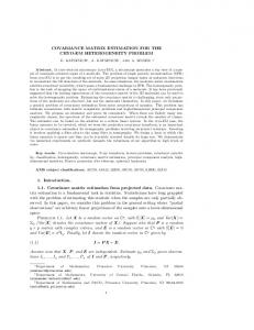
servations, forecast accuracy would be a function of predictability limits only. If, on the other hand, model error is signi cant | as has been suggested by a number of studies (Boer, 1984; Bloom & Schubert, 1990), then its eect on forecast error must somehow be accounted for when forecast and observations are combined into an analysis. Cohn (1993) has shown, for dynamics governed by a scalar hyperbolic partial dierential equation, that important forecast error characteristics such as correlation length scales can be strongly in uenced by their model error counterparts. Quantitative information about model error must be obtained before it can be determined how and whether sophisticated statistical data assimilation techniques can be successful in actual operational systems. If the in uence of model error on forecast error is important, yet complete model error statistics are unknown, then forecast error covariance computations will always turn out to be approximate at best | regardless of the way in which propagation of initial error is accounted for. Given the extent (or lack) of our knowledge of model error, how accurately should one attempt to account for propagation of initial error? This question is especially interesting since covariance propagation represents by far the most expensive step in the Kalman lter algorithm. Finally, how much do we really need to know about forecast error and/or model error in order to produce accurate analyses? 3000 sample rms errors (incorrect model error parameters) sample rms errors (correct model error parameters)

2000

1000

1

2

3

4

5

6

Figure 1: Rms energy error evolution for SKF with misspeci ed (upper part) and correctly speci ed (lower part) model error statistics. Marks indicate actual rms errors, curves correspond to their statistical expectations. In Figure 1 we show an example of the possible eect on lter performance of incorrectly speci ed model error statistics. The plot shows the time evolutions of the rootmean-square (rms) energy error for two data assimilation experiments, performed with the two-dimensional linear shallow water model of Cohn and Parrish (1991). The curves correspond to statistical expectations of forecast and analysis errors (obtained from Kalman lter theory), while the marks denote the errors that actually occurred. In each experiment the same 12-hourly batches of synthetic radiosonde observations were assimilated into a forecast model by means of a simpli ed Kalman lter (SKF) (Dee, 1991). The two experiments dier only in the way that model error covariance is speci ed. The rms-error curve and marks in the lower part of the gure result from a correct speci cation of model error covariance, while those in the upper part result from misspeci cation. The disastrous eect of erroneous model error information is clearly visible. The average analysis error level more than doubles after a few days of assimilation. In some cases (at 0.5, 1.5, and again at 5.5 days) the assimilation of observations actually has a negative impact on the analysis! 3

Only two model error covariance parameters play a role in this example. The misspeci cation consists of an overestimation of model error signal strength by a factor of 2, and underestimation of the model error correlation length, again by a factor of 2. All other statistical properties of model error are speci ed correctly, including stationarity and whiteness, the fact that model error acts exclusively on the slow subspace of the forecast model, and a great deal of other statistical information. These and other details pertaining to this numerical example will be given in Section 6. Covariance parameters such as those that play a role in this example can actually be estimated on the basis of the same observations used for producing the analyses. In the context of estimation theory, a number of adaptive ltering approaches have been developed and applied with varying degrees of success to real-life problems (see Moghaddamjoo and Kirlin (1993) for a recent survey). However, the available methods tend to be either excessively expensive to implement in a large, real-time data assimilation system, or they are inapplicable to begin with because they apply to highly specialized situations only. In this paper we present a simple approach to on-line covariance parameter estimation, speci cally designed for a situation in which the number of available observational data for an analysis is much larger than the number of tunable covariance parameters. Thus, our scheme can be used to produce on-line estimates of certain basic error covariance parameters which are currently unknown. Incorporation of the scheme into a statistical data assimilation method will force those parameters to remain consistent with the actual observations. While this will only ful ll part of the total information requirement for a Kalman lter, it should help to improve the performance of practical implementations of statistical data assimilation schemes. Before presenting the parameter estimation scheme, we clarify in Section 2 what we mean by model error. We do this in order to explain that certain important assumptions usually made in applying estimation theory are generally false in practice. As a consequence, even a full- edged nonlinear extension of the Kalman lter can do no better than to roughly approximate actual forecast error covariance evolution in an operational setting. It will follow that the model error statistics supplied to a Kalman lter should be viewed as the calibration parameters for the algorithm, to be tuned on observational data. Calibration of model error statistics is problematic since the totality of observational information at any give time is insucient to estimate even the state of the atmosphere, let alone a complete set of model error covariances. This necessitates the introduction of parameterized model error representations in order to reduce the number of degrees of freedom. We brie y review a few of these representations in Section 3, and derive an expression for the covariance of observed-minus-forecast residuals which provides the basis for on-line estimation of the covariance parameters. In Section 4 we present a maximum-likelihood scheme for producing parameter estimates from a single batch of observations at a particular time instant. This estimation scheme can be incorporated into a four-dimensional data assimilation cycle in various ways, in order to produce on-line, time-dependent estimates of model error and/or observation error parameters which are continously adjusted based on current observations. We brie y outline application to the SKF and to OI in Section 5. We report in Section 6 on some numerical experiments with an adaptive SKF and with an adaptive version of OI, using the linear two-dimensional shallow-water code of Cohn and Parrish (1991). Although the model is extremely simple compared to actual operational forecast models, we include some rather interesting examples in order to demonstrate that the adaptive scheme can perform well in a wide range of circumstances. In Section 7 we brie y conclude.

4

2 Model error In the introduction we de ned model error to be the contribution to forecast error which is due to dierences between the forecast model and the actual atmosphere. Estimation theory represents these dierences by additive stochastic perturbations: the actual atmosphere is presumed to behave like a noisy version of the forecast model. The situation in reality can be expected to be more complicated. Consider rst a linear forecast model. Numerical integration over one model timestep can be expressed by the dierence equation (1) wfk = fk;k?1 wfk?1 ;

where f represents the forecast model in operator form, and w f denotes the forecast. Depending on the time index k, the input wfk?1 can be an analysis or a previous forecast, but that is not important here. Let us assume for the moment that the actual atmosphere is governed by a well-posed system of partial dierential equations. Its evolution from time tk?1 to tk can then be described by the equation wtk = tk;k?1wtk?1 ; (2) where t stands for the (unknown) solution operator associated with the governing PDE (see Cohn and Dee (1988, Sec. 2)), and wt denotes the (in nite-dimensional) state of the atmosphere. Throughout this paper, vectors w represent atmospheric states or approximations thereof. All quantities with superscript t are associated with the actual (true) atmosphere, and are therefore unknown. Forecast error can be de ned once we have a way of comparing ( nite-dimensional) forecasts with (in nite-dimensional) actual states. We introduce a projection operator  for this purpose and let (3) we fk  wfk ? wtk ; where we f denotes forecast error. Applying the projection operator to (2) and then subtracting the result from (1) gives the following equation for the evolution of forecast error:

we fk = fk;k? we fk? +
k;k? wtk? ; where
is the operator given by
k;k?  fk;k?  ?  tk;k? : 1

1

1

(4)

1

(5) Equation (4) shows clearly the two sources of forecast error. The rst term on the right-hand side expresses error propagation by a known, nite-dimensional operator. The second term represents model error, and involves unknown operators and quantities only. So far we only considered model error which is due to the discrepancy between the (linear) forecast model operator f and the evolution operator t associated with the actual atmosphere, which we took to be deterministic. A nonlinear version of (4) would contain an additional term representing linearization errors. There may be other, equally intractable sources of model error due to (possibly stochastic) external forces which are not represented by the forecast model at all. The expression for model error appearing in (4), however, shows that the combined eects of model de ciencies (e.g. parameterizations of physical processes, nite resolution) depend nonlinearly upon the actual state of the atmosphere in an unknown manner. 1

1

1

5

by

In the Extended Kalman lter (EKF), the forecast error evolution equation (4) is replaced

(6) we fk = Afk;k? (wfk? )we fk? + G(wfk? )ebtk ; where Afk;k? is the tangent linear model operator associated with the nonlinear forecast model. The term G(wfk? )ebtk represents model error; the operator G as well as the properties of the stochastic process febtk g are to be speci ed. Note that G represents the available 1

1

1

1

1

1

deterministic knowledge about model error; it is often taken to be the identity. Replacing model error by an additive stochastic perturbation as in (6) is in fact a modeling device, used to represent the combined eects of the various model error sources mentioned earlier. In addition, many simplifying assumptions about the stochastic sequence febtk g are usually introduced in actual EKF applications. Typical assumptions are whiteness (statistical independence of successive noise terms), stationarity (constancy in time of all statistics), absence of bias (statistical mean is zero) and normality (a Gaussian joint probability distribution of all elements of the noise process). All of these can be relaxed in theory; to do so, however, would lead to more complicated algorithms with additional information requirements. In practical applications most of this information is unavailable. The point of this exposition is to show that estimation theory provides a framework which contains inherent approximations, particularly regarding the representation of model error. Application of the theory requires additional approximations. Equation (4) clearly shows that model error indeed depends on the actual atmospheric state, which implies that the assumptions that are usually made in applying the theory | e.g., to derive an EKF | are questionable. This remark has important consequences for the design of model error estimation algorithms, as we shall explain below. Still, the EKF error evolution equation (6) may well represent the best we can do in terms of forecast error modeling, particularly since a more sophisticated scheme would lead to additional information requirements. Replacing model error by a stochastic perturbation to the forecast model is conceptually defensible in view of the multitude of unknown error sources. In view of the previous discussion, however, it would seem that actual implementations of the EKF should incorporate state-dependent model error statistics. Let us therefore stick with the EKF for the moment, and consider the error covariance evolution associated with a forecast: (7) P fk = Ak;k?1 P fk?1ATk;k?1 + GQk GT where (8) P fk  E [we fk (we fk )T ] Qk  E [ebtk (ebtk )T ] (9) denote forecast and model error covariances; E is the expectation operator (Jazwinski, 1970, p. 19). Equation (7) is obtained directly from (6) under the assumption that

E [we fk?1 (Gebtk )T ] = 0 ;

(10)

i.e., current model error is independent of previous forecast error. In view of the remarks just made, the EKF error covariance evolution equation (7) must be taken with a grain of salt. It is simply a means for representing forecast error covariance, which accounts in an approximate manner for the eects of error propagation by the forecast model as well as for additional eects of model error. Since the underlying assumptions are actually violated, the unknown quantities in the equation should be regarded as calibration parameters which do not necessarily have any physical meaning. 6

The unknown quantities in the recursion (7) are, of course, the family of covariance matrices fQk g. In addition, the equation must be initialized with a speci cation of P fk at some time tk = t0 . Usually the recursion will start from an analysis, so that P f0 = P a0 , an estimate of the analysis error covariance. It can be shown that under certain conditions the eect of misspeci cation of P f0 will disappear, provided a sucient number of observations are assimilated during a suciently long period of time (Jazwinski, 1970, Theorem 7.5). Speci cation of fQk g would require a gigantic amount of information, which is generally not available. The only data from which model error covariances could possibly be identi ed are observational. Since the number m of meteorological observations at any given time is much less than the number n of degrees of freedom of a forecast model, it is not possible to estimate all required parameters for specifying model error covariance. This is true regardless of the estimation procedure used since the number of such parameters is n(n+1)=2 per time step | several orders of magnitude larger than m. Apart from this practical limitation on the number of parameters that can be identi ed from the available observations, there may be theoretical limits as well. For example, Mehra (1970) has shown, for the special case of a linear model with stationary model error (i.e., model error statistical properties are independent of time, so that Qk = Q) and stationary observation operator (i.e., the same type of observation is made at each time step), that at most nm model error covariance parameters can be identi ed from an in nite time series of m observations per time step. The only feasible approach is therefore to severely reduce the number of degrees of freedom by parameterization, and then to try to estimate the parameters. In view of the fact that the representation of model error in the EKF framework by a stochastic perturbation to the forecast model is approximate to begin with, this is also the only sensible approach. It then follows naturally that other approximations can be legitimately introduced in the EKF forecast error covariance evolution equation (7), particularly in the computationally expensive propagation term. The result will be a severely simpli ed representation of forecast error covariance. An interesting question is whether this can be eective | that is, whether the representation will be adequate for the purpose of producing accurate analyses. If the forecast model is suciently accurate, misspeci cation of model error covariance might not seriously aect analysis accuracy. On the other hand, the example presented in the Introduction indicates that misspeci cation of model error covariance can have a signi cant negative impact indeed.

3 Covariance parameterization Parameterizations of model error covariance can be obtained by formulating a set of hypotheses about model error characteristics, and using these to derive an expression for model error covariance Qk = Qk () (11) which depends on a vector  of unknown parameters. Once such a parameterization has been constructed, (11) represents a model for model error covariance and the objective is to calibrate this model on the basis of available observations. A special class of parameterizations is obtained by assuming model error to be stationary, i.e., Qk = Q() : (12) This reduces the number of degrees of freedom considerably, and opens up the possibility to develop o-line procedures for estimating parameters in Q or possibly Q itself (Daley, 1992a). Although it is not clear what precisely would be estimated in case model error is not actually stationary, it would seem that much can be learned about the stationary 7

component of model error from such a procedure. This, in turn, might lead to new and improved nonstationary parameterizations. An adaptive Kalman lter was developed by Belanger (1974) for a special case of (12), and its possible application to the atmospheric data assimilation problem was explored by Dee (1983). Belanger showed how to estimate  = ((1); : : :; (N )) in N

Qk = Q = X  i Q i ; ( )

(13)

( )

i=1

with Q(i) known, meaning that model error is stationary and that its covariance can be expressed as a linear combination of known component matrices. An ecient version of the Belanger algorithm (Dee et al., 1985) applied to a simpli ed Kalman lter (Dee, 1990; Dee, 1991) could be computationally feasible for atmospheric data assimilation. However, this adaptive lter relies strongly on unrealistic assumptions (model linearity and model error stationarity) so that it may not work very well in practice. Furthermore, the type of parameterization (13) is not convenient for estimating parameters which appear nonlinearly in Q. Another type of model error parameterization was introduced by Cohn and Parrish (1991) for the purpose of setting up their Kalman lter experiments with a linearized shallow-water model. This parameterization was derived from the hypothesis originally put forward by Phillips (1986) that forecast error consists of an ensemble of mutually independent slow modes of the forecast model. Phillips' hypothesis is supported in part by diagnostic studies of ECMWF forecast error elds (Hollingsworth & Lonnberg, 1986); Cohn and Parrish (1991) have provided some additional theoretical justi cation as well. For a linear forecast model, the resulting covariance parameterization can be expressed as (14) Qk = V S Qb k ()V S ; where V S is the matrix whose columns are the slow modes of the forecast model and V S is its Hermitian transpose. The diagonal matrix Qb k () is the model error spectrum, meaning that its nth diagonal element is the variance of the nth modal expansion coecient of model error. Surely when approximate schemes for computing forecast error covariance evolution have developed to the point where they can be made computationally feasible in an operational setting, model error parameterization will start to receive a great deal of attention and more re ned parameterizations than (14) will be proposed. Work is currently underway (Cohn, personal communication) toward parameterizing the speci c contribution to model error caused by discretization of the governing PDE. Other known sources of model error can perhaps ultimately be analyzed as well and accounted for by means of a parameterized covariance contribution. Some operational versions of Optimal Interpolation actually contain parameterized representations of model error, although it is not usually explicitly formulated as such. Forecast error covariances are computed in these systems by imposing a xed correlation structure and by prescribing the height error increments
he : the increase in height error standard deviation which is expected to occur during the course of an assimilation cycle. Height error increments can be parameterized in dierent ways | for example, they can be made to depend on latitude and vertical level only; in general,
he k =
he k () : (15) Depending on the details of the OI implementation, the quantity
he k can be formally related to model error covariance Qk . See Todling and Cohn (1994) for a clear explanation of the precise way in which the height error increments can be used in dierent versions of OI 8

to construct the forecast error covariance. When we refer to model error parameterization below, we include the possibility of height error increment parameterization as well. Regardless of the particular technique employed, parameterizing model error covariance in a statistical data assimilation scheme leads to a parameterized representation of forecast error covariance: P fk = P fk () : (16) That is, for any given model error parameterization, a speci c choice of the parameters  completely determines the model error covariance, which in turn leads to a completely speci ed forecast error covariance. The precise details of this last step depend on the data assimilation method, particularly on the way in which covariance propagation is represented. Taking it one step further, model error parameterization in fact amounts to a parameterization of the covariance of the innovations vk , given by (17) vk  wok ? Hk wfk ; where wok denotes the vector of observations and Hk is the observation operator at time tk . The observation operator is simply a device for comparing forecast model output with observations, generally nonlinear but essentially known; its precise formulation depends on the type of observing instruments it represents as well as on the forecast model. Using the de nition of forecast error (3), the innovation can be written

vk = we ok ? Hk we fk where we o is the observation error de ned by we ok  wok ? Hk wtk ;

(18) (19)

with  the projection operator introduced in the previous section. From (18), the innovation covariance is given by

E [vk vTk ] = E [Hk we fk (Hk we fk )T ] + E [we ok (we ok )T ] ? E [we ok (Hk we fk )T ] ? E [Hk we fk (we ok )T ] :

(20) This expression can be approximated by linearizing the observation operator and neglecting cross-correlations between forecast and observation errors. This results in (21) E [vk vTk ]  H k P fk H Tk + Rk ; with H k a linearized version of Hk , and Rk the observation error covariance: (22) Rk  E [we ok (we ok )T ] : At rst glance it might seem that observation error statistics are easier to determine than forecast error statistics. Examination of (19), however, shows that this is by no means self-evident. For example, it is not straightforward to determine error characteristics associated with observation operators involving models that stipulate the relationship between forecast model quantities (e.g., temperatures) and observed quantities (e.g., radiances); see Daley (1993). Let us therefore allow for the possibility of parameterizing observation error as well, i.e., Rk = Rk ( ) (23) with a vector of unknown observation error parameters. Actual observation error statistics are probably state-dependent, just as model error statistics are. 9

In any case, parameterization of model error (11) and possibly observation error (23) ultimately leads to a parameterization of the innovation covariance: (24) E [vk vTk ]  H k P fk ()H Tk + Rk ( ) : This expression provides the basis for on-line estimation of the model error parameters  and/or the observation error parameters , as follows. Suppose, for the moment, that  and are xed. All statistical data assimilation schemes actually compute the innovation covariance expressed by the right-hand side of (24); this is done during each analysis in order to determine the weighting coecients in the analysis update. On the other hand, the actual innovations v k are available as well; they are simply the forecast-minus-observed residuals produced by the system, cf. (17). By monitoring the innovations one can check whether the system's innovation covariance representation | the right-hand side of (24) for xed , | is in fact consistent with the actual innovations; see also Daley (1992b). We will show in the next section how this can be done without any signi cant computational expense. Next, consider  and/or unknown. Then the right-hand side of (24) represents a family of innovation covariances rather than a xed one. It is still the case that the actual innovations v k are available on-line. Therefore one can attempt to locate a particular member of the parameterized family of covariance representations (i.e., nd a set of parameter values) which is consistent with the actual innovations being produced by the data assimilation system. This method is known as covariance matching; see Moghaddamjoo and Kirlin (1993, p. 70). A criterion for consistency will have to be formulated, and this will lead to an optimization problem for the unknown parameters. Thus the parameters  and/or can be estimated by calibrating the covariance model on the right-hand side of (24) to the actual innovations. The general approach outlined here can be implemented in many dierent ways, depending on the form of the covariance parameterization, on the particular data assimilation scheme, and on the criterion for optimization. If the number of unknown parameters is a small fraction of the total number of observations available for an analysis, then it should be possible to obtain parameter estimates instantaneously, just prior to the analysis. We will explain this in some detail in Section 5. An important advantage of such an approach is that it permits time-dependent parameter estimates which are continuously adjusted on the basis of current observations. If model errors and/or observation errors are in fact strongly statedependent, this might very well be a crucial requirement for an adaptive data assimilation scheme which is to perform satisfactorily in an operational setting.

4 Single-sample parameter estimation In the previous section we showed that model error and/or observation error parameterizations imply a parameterization of the innovation covariance, and that this can provide the basis for covariance parameter estimation. We have also argued that it should be possible to estimate parameters using a single innovation sample | that is, the actual innovation produced by a data assimilation system at a single analysis time. In this section we will therefore consider one particular but arbitrary time instant at which an innovation v is produced, and assume that we have a covariance model for v which involves a number of unknown parameters: E [vvT ]  S () ; (25) where S () is a family of known covariance matrices parameterized by . In order to simplify the notation we removed the time index k and no longer distinguish model error parameters from observation error parameters: S () replaces the right-hand side of (24). 10

One way to calibrate the covariance model S () to the innovation sample v is by producing the maximum-likelihood estimate of  (Burg et al., 1982). For this purpose we introduce the assumption that v  N (0; S()) (26) for some  =  , i.e. the innovation is a normally distributed, zero-mean random vector whose covariance is the matrix S ( ). The conditional probability density p(vj) of this random vector is then given by the Gaussian density function   p(vj) = (2)? m (det S())? exp ? 12 (vT S ?1 ()v) : (27) where m = dim v. Given the innovation sample v , the maximum-likelihood parameter estimate ML of  is obtained by nding that value of  for which the probability density (27) attains a maximum: ML = arg max  p(vj) = arg min (28)  f () 2

1 2

where

f () = log det S () + v T S ?1 ()v

(29)

is the maximum-likelihood function obtained from the natural logarithm of (27). Minimization of (29) corresponds to nding the most plausible value of the parameter vector , given the observed sample v. The maximum-likelihood criterion is simply a device for matching the covariance model S () with that which is observed. An assumption about the distribution of v such as (26) is required to formulate the criterion; however the validity of this assumption is not essential. If the innovation v is not in fact normally distributed, or if its covariance is not of the form S () for any , then the estimate obtained by minimizing the function (29) will not be truly a maximum-likelihood estimate. Nevertheless, the eect of calibrating the parameters  in this manner will be to improve the consistency between the parameterized covariance model and the actual innovations. We use the following simple example of single-sample maximum-likelihood estimation to illustrate these remarks. Suppose that the innovation covariance parameterization is linear in a single parameter: S () = S 0 (30) with S 0 a xed covariance matrix and  an unknown scalar. In this case optimization of the maximum-likelihood function (29) can be performed analytically as follows. From f () = log det(S 0) + vT (S 0)?1 v = m log  + log det S 0 + 1 v T S ?0 1 v (31) we nd



df m 1 T ?1 d =  ? 2 v S 0 v : The minimum of f () is therefore attained when  = ML = m1 vT S ?0 1 v :

(32) (33)

11

This means that, based on a single sample of the innovation v, the best (in the maximumlikelihood sense) scaling of S 0 is given by E [vvT ]  MLS 0 : (34) with ML given by (33). In general, the statistical properties of the parameter estimate ML depend upon the actual probability distribution of the innovation v. If, in fact, v  N (0; S 0) ; (35) for some (unknown) parameter value , then the probability density of ML can be obtained in closed form. In Dee (1992) it is shown that (33,35) imply

ML



 m m  ? 2 ; 2 ; 

(36)

that is, ML has a gamma distribution and its mean and variance are given by E [ML] =  ; E [(ML ? )2] = 2 m2 :

(37) (38)

The maximum-likelihood estimate ML pis therefore unbiased, and its standard deviation relative to the true value  is given by 2=m. For example, 10% relative accuracy can be obtained with 200 observations; 5% relative accuracy with 800 observations. In reality, the actual covariance of innovations is not likely to be a member of the postulated family of covariances S () and its probability density may be dierent from Gaussian. Without additional information, however, there is no obvious way to improve the estimate (33). In order to analyze this case, suppose that, instead of (35), the actual probability density of the innovation v is unknown. Suppose that E [v] = 0 (39) T E [vv ] = S (40) for some unknown covariance matrix S . Then we have E [ML] = 1 E [vT S ?1 v] =

m X i;j

0

(S ?0 1 )ij S ij

1 trace hS ?1 S i : = m 0

(41)

Thus, the estimate ML can generally be interpreted as a scaling factor. Replacing the covariance S 0 by the scaled version ML S 0 forces the expression (41) to equal unity. This has the eect of bringing the parameterized covariance model S 0 as closely as possible to the actual covariance S | `close' in a sense which can only be made precise, however, in terms of the unknown covariance S . The simple analytical example just presented is of practical interest as well, for it can be used almost trivially to monitor the consistency between a data assimilation scheme's representation of the innovation covariance on the one hand, and the information contained in the actual observations on the other. If we take the matrix S 0 to be the innovation covariance as constructed by a statistical data assimilation scheme, then the parameter estimate given by (33) produces a scaling factor that, according to maximum-likelihood theory, should multiply S 0 in order to improve the consistency between the scheme's covariance model and the actual data. This scaling factor can be used as a diagnostic, since it must be close to 12

unity for the covariance model to be correct. If, say, the scheme overestimates innovation covariance, then the scaling factor will tend to be smaller than unity. Thus, by monitoring a time series of scaling factors, one can learn whether the scheme consistently under- or overestimates innovation covariance. Calculation of the scaling factor can be performed in operational implementations of statistical data assimilation schemes at insigni cant cost. The quantity S ?0 1 v is usually computed as an intermediate step in order to produce the analysis increment, so that only an inner product of length m (the number of observations) is required in order to compute (33). Currently operational versions of OI compute the analyses in limited subdomains of the model's total spatial domain. A separate scaling factor can then be computed for each analysis box, and its values would show whether or not the OI representation of the innovation covariance within each box is reasonably scaled with respect to the actual observations within that box. Some preliminary experiments of this type have been performed with the HIRLAM analysis system (Kallberg, 1989); results will be reported elsewhere. In the general multi-parameter case, minimization of (29) with respect to  is computationally expensive. Depending on the optimization method used, the maximum-likelihood function f () and possibly its gradient will have to be evaluated repeatedly. As shown in Dee (1992), the gradient of f is given by

@f = trace S ?1 ? S ?1 vv T S ?1  @ S  ; @(i) @(i)

(42)

where @@ i S denotes the matrix obtained by dierentiating each element of S () with respect to (i) , the ith element of . Given S () and v, evaluation of f () requires factorizing S and computing S ?1 v . These calculations correspond to what is usually done in an analysis update. The cost of the rst evaluation of f () is therefore nil. A gradient evaluation, on the other hand, requires computation and storage of S ?1 and @@ i S . Whether or not this is feasible depends primarily upon the nature of the parameterization. However, the greatest cost of the optimization process may be involved in re-computing the innovation covariance model S () for dierent values of . Each re-evaluation of the maximum-likelihood function f () for a new value of the parameter vector  essentially amounts to a repeated calculation of the forecast error covariance and/or observation error covariance; see (24). How this is done and how expensive it is to do so depends, of course, on the form of the parameterization as well as on the particulars of the data assimilation method. In the next section we will outline the procedure for a simpli ed Kalman lter and for those versions of OI which incorporate height error increments. ( )

( )

5 Application to four-dimensional data assimilation In the previous section we showed how estimates of innovation covariance parameters can be obtained from a single batch of simultaneous observations. All statistical data assimilation methods compute, in one way or another, approximations to the innovation covariance. The single-sample parameter estimation scheme does not rely on the speci c way in which this is done; it is therefore relatively easy to incorporate into four-dimensional statistical data assimilation methods. In this section we outline the application to the simpli ed Kalman lter (SKF) and to Optimal Interpolation (OI). Complete descriptions of these methods can be found in the references given in the Introduction. Here we only sketch brie y the forecast error covariance representation associated with each method, and show how they can be adjusted to the observations just prior to producing an analysis. 13

5.1 Adaptive SKF The basic idea behind the SKF is to predict forecast error covariance evolution by means of a simpli ed version of the forecast model itself | unlike the Kalman lter, in which the full forecast model is used for error prediction. If the essential aspects of error dynamics can be captured by the simpli ed error model, the resulting loss of accuracy should be acceptable in view of the many other approximations and lack of information inherently associated with the Kalman lter. An SKF for the shallow-water equations was proposed by Dee (1991), with forecast error prediction based on advection of height errors combined with geostrophically balanced wind errors. Todling and Cohn (1994) experimented with this scheme in the context of a linear two-dimensional shallow-water model, and showed that a more sophisticated type of covariance balancing must be introduced in order for the SKF to work well in that case. The SKF forecast error covariance prediction step can be described as follows. Just prior to computing an analysis at time tk , an approximation S fk to the actual forecast error covariance P fk is produced. This approximation is based on (i) an approximation S ak?l to P ak?l , the actual SKF analysis error covariance at the previous analysis time tk?l , and (ii) an approximation Q (b k ) to Qk , the actual model error covariance. This is expressed by a SKF b ) ; S fk = 'SKF k k;k?l (S k?l ) + lQ (

(43) where the symbol 'SKF k;k?l represents the sequence of operations accounting for covariance propagation and balancing. Note the factor l multiplying QSKF k , which is supposed to account for the accumulation of model error during the l model time steps comprising the forecast period. The SKF becomes adaptive when b k is made to depend on actual observations. This is done, as described in the previous section, by tuning the innovation covariance S () = H k S fk ()H Tk + Rk a T SKF T = H k 'SKF (44) k;k?l (S k?l )H k + Rk + lH k Q ()H k ; to the actual observations. More precisely, when observations wok become available at time tk , the innovation vk = wok ? H k wfk is computed; subsequently the maximum-likelihood function (29) is minimized with S () given by (44). This optimization procedure produces the maximum-likelihood estimate ML k of the model error parameter vector  based on the observations at time tk . This estimate (or a smoothed version of it; see below) can then be used in (43) to update the SKF model error covariance representation. This will result in a more realistic forecast error covariance, which, in turn, should improve the analysis.

5.2 Adaptive OI Some operational implementations of OI (McPherson et al., 1979; Schubert et al., 1993) (i) approximate forecast height error variances by adding xed increments
he k to the estimated height error variances associated with the previous analysis, and (ii) construct a full, multivariate forecast error covariance based on prescribed cross-correlation functions. This can be expressed by (45) S fk = 'OIk;k?l(S ak?l;
he (b k )) ; where the symbol 'OI k;k?l represents the sequence of operations needed for the OI multi-variate forecast error covariance construction. Such a version of OI can be made adaptive by calibrating
he (b k ) to the available observations at time tk . Equation (45) implies a parameterization of the innovation covariance, 14

now given by S () = H k S fk ()H Tk + Rk a T e = H k 'OI (46) k;k?l (S k?l ;
h())H k + Rk : A maximum-likelihood estimate kML of the height error increment parameter vector  based on the observations at time tk can then be obtained as before, by minimizing the maximumlikelihood function f () given by (29), with S () now as in (46). Some implementations of OI, as well as SSI and 3DVAR, do not rely on prescribed height error growth increments to approximate forecast error covariances, but utilize stationary covariance information instead. Such information generally depends on covariance representations which are somehow parameterized, and it should not be dicult to produce on-line estimates of the parameters involved using the single-sample maximum-likelihood approach.

5.3 Optimization of the maximum-likelihood function For our numerical experiments we performed a simple golden-section search (Gill et al., 1981, p. 90) in order to nd the maximum-likelihood parameter estimates. This means that the innovation covariance S () must be constructed repeatedly for successive trial values of the parameter vector , until a minimum of the maximum-likelihood function f () is found. Clearly this approach can only be used for estimating one or two parameters; higherdimensional optimization requires a more sophisticated, gradient-based technique. Computational cost will certainly be an issue, since each additional evaluation of the maximumlikelihood function costs about the same as computing an analysis, and gradient evaluations are even more expensive. Note, however, that it is probably not worthwhile to expend an enormous computational eort in order to calculate the maximum-likelihood estimate to within an accuracy of, say, better than 10{20%. As we discussed in the previous section, the estimates themselves are random; the probability density upon which the maximum-likelihood estimate is based may not in fact be Gaussian; and the eect on actual analysis errors of small perturbations in  may be negligible anyway. Rough estimates of covariance parameters can be obtained on the basis of a few hundred observations per parameter. In a boxed OI system, for example, one could estimate one or two parameters per analysis box by means of a simple search method. This would result in local (in space and time) parameter estimates, which can then be used to improve the forecast error covariance representation within each analysis box.

5.4 Smoothing For a variety of reasons it may be desirable to apply some kind of smoothing (in space and/or time) of the maximum-likelihood estimates. In the numerical examples shown in the next section we use smoothing because the number of available observations in these experiments is relatively small, so that single-sample parameter estimates tend to oscillate. In a more realistic data assimilation system with a larger number of available observations, smoothing of the estimates might still be desirable. For example, as we shall see in one numerical example below, oscillations in the sequence of single-sample estimates may be due to ill-posedness of the covariance estimation problem. In our experiments we use the simple one-step smoother scheme given by ML b k = (mbmk?l ++ mmk ) ; (47) where b k denotes the smoothed estimate at time tk , kML is the single-sample maximumlikelihood estimate at time tk , and m is an integer which controls the amount of smoothing; 15

recall that m = dim vk is the number of observations in the single sample. The smoother is initialized with b 0 = 0 , the a priori (generally misspeci ed) parameter values that the data assimilation scheme is supplied with. b k?l The smoothing algorithm given by (47) can be motivated as follows. Both ML k and  may be thought of as estimates of  , the actual (or optimal) model error parameters. If, based on the simple one-parameter example worked out in the previous section, we conjecture E [jjML ?  jj2] / 1 ; (48) k

m



(see (38)) and, in addition, that E [jjb ?  jj2] / 1 ; k?l



(49)

m

for some integer m, then one can easily show that (47) provides the minimum-variance estimate of  . Note that the degree of smoothing increases with m; no smoothing occurs when m = 0.

6 Numerical experiments All experiments reported here utilize the linearized two-dimensional shallow-water model of Cohn and Parrish (1991), combined with arti cially generated model error. This setting was recently used by Todling and Cohn (1994) (to be referred to as TC94 in this section) in order to study various approximations of the Kalman lter equation for forecast error covariance evolution. The Kalman lter itself does not involve any approximations in this situation, since all underlying assumptions about model error etc. are satis ed by design. TC94 concerns the methodology of forecast error covariance evolution, and speci cally addresses various ways to propagate error covariance by model dynamics. In order to allow for a fair comparison among the various schemes they considered, each was supplied with full information about model error and observation error statistics. In this work, however, we are concerned with the eects of misspecifying error statistics, and with a means for correcting such eects. We therefore repeat some of the experiments from TC94, speci cally those with the balanced SKF (denoted by SKF below) and the balanced OI with zonally averaged growth rates (referred to as OIZ below). However, in each experiment we change the speci cation of certain statistical parameters and subsequently attempt to estimate those parameters on-line.

6.1 Experimental design The implementation of the forecast model used for our experiments is described in TC94 (Section 2 and Table 1). The evolution of the actual atmosphere is simulated by applying a random perturbation to the forecast model at each model timestep; i.e.,

wtk = f wtk? + ebtk (50) where f represents one timestep of the forecast model's nite-dierence operator and ebtk 1

denotes model error. A random number generator is used to produce a normally distributed, white model error sequence with zero mean and covariance of the form

E [ebtk (ebtk )T ] = Qk = V S Qb ( k ; Lk)V S ;

(51) as in (14). The columns of the matrix V S contain the forecast model's slow modes; consequently model error is restricted to the slow subspace. The matrix Qb is taken to be diagonal: Qb ( k; Lk ) = diag(qb(nj ; k; Lk )) (52) 16

with nj the two-dimensional wavenumber associated with the j th slow mode of the forecast model, and qb is the Gaussian model error spectrum given by ! "  2 # 2  L n 0n k 2 qb(n; k; Lk )) = k 1 + f 2 a2 exp ? 2a : (53) 0 Here 0 is the mean geopotential height of the basic ow about which the shallow-water equations are linearized, f0 is the Coriolis parameter at the central latitude of the model domain, and a is the radius of the earth. See Cohn and Parrish (1991, Eqs. (4.30{4.34)) for a detailed description of this spectrum. In particular, it is shown there that (53) corresponds to height error correlations which are roughly Gaussian, with correlation length Lk . The parameter k determines the amplitude of the spectral peak. In most of our experiments, both model error spectrum parameters k and Lk are xed constants as in TC94:

k =  ; (54) Lk = L : (55) We show the results of one experiment below in which actual model error statistics are made to be time-dependent by letting the amplitude parameter k vary in time. We also include an experiment in which the probability distribution of model error is uniform, rather than normal. Twelve-hourly radiosonde observations of the three model variables h; u, and v at 77 locations are generated as in TC94 by adding random measurement errors to the (simulated) actual values of the variables at those locations. Therefore 231 observations are available at each analysis time, which should be sucient for estimating one covariance parameter on the basis of a single set of observations. When we try to simultaneously estimate multiple parameters, the variance of each single-sample estimate tends to be rather large. This can be alleviated by applying a smoother to the single-sample estimates, as described in Section 5.

6.2 Adaptive SKF experiments In our rst set of experiments the SKF is provided with an initial misspeci cation of the model error spectrum parameters  = ( ; L). We take  SKF b (56) QSKF k = Q (k ) = V S Q( k ; Lk )V S ; but with

0 = 2  ; (57) L0 = 0:5L : (58) Figure 1, brie y discussed in the Introduction, shows what happens to the rms forecast and analysis errors when the model error parameters are held xed at  = ( 0; L0). In subsequent gures the rms error statistics for this non-adaptive SKF with incorrectly speci ed model error statistics will be reproduced in order to provide a basis for comparison with the adaptive schemes. Also plotted in Figure 1 is the rms error evolution for the case  = ( ; L), i.e. the SKF with correctly speci ed model error parameters. As shown by TC94, the performance of the SKF in this case is virtually indistinguishable from that of the (optimal) Kalman lter, so that it provides a lower bound for the statistical rms error levels that can be attained by any data assimilation scheme in this experimental setting. In subsequent gures we therefore include the rms error curve associated with this non-adaptive SKF with correctly speci ed model error statistics as well. The sample rms errors shown in this and further gures represent domain-averaged dierences between the forecast and the actual atmospheric state, simulated by means of (50{55). 17

In order to save space we show only the total energy of this dierence; plots of the rms errors in the individual model variables u; v , and h tend to look rather similar. Note that these sample errors are random: they correspond to a single realization of the stochastic-dynamic model (50). Many of our experiments were repeated for a number of dierent realizations (i.e., dierent seeds for the random-number generator), resulting in slight variations in the sample rms errors. For example, the tendency for sample errors to be smaller than their statistical expectation during the last 24 hours in Figure 1 turns out to be a feature of that particular realization. The solid curves shown in Figure 1 indicate statistical expectations of the sample rms errors, obtained by computing the actual error covariance evolution for the experiment (see e.g. TC94). Actual error statistics for the adaptive experiments reported below can not be computed in this manner, since the forecast and analysis errors of an adaptive scheme are generally state-dependent. This violates one of the assumptions needed for the covariance computation. In our adaptive experiments we will therefore look at sample rms errors, together with the estimated rms error statistics produced by the assimilation scheme itself. Actual error statistics could be computed using a Monte-Carlo approach. 3000 estimated rms error statistics sample rms errors

2000

1000

2 single-sample estimates statistically smoothed estimates 1

1

2

3

4

5

6

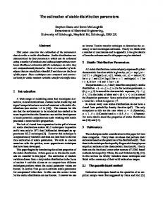
Figure 2: Rms energy error evolution and model error parameter estimates (normalized by ) for Experiment ASKF-I. The solid curves are reproduced from Fig. 1. In our rst parameter estimation experiment (Experiment ASKF-I) we calibrate only. This means that the lter will attempt to adjust the model error spectral amplitude while working with the wrong type of spectrum, since the correlation length scale is held xed at the erroneous value L0 . With this type of experiment we try to emulate what might happen when the shape of the actual model error spectrum is unknown to begin with. Figure 2 shows the evolution in time of the rms errors produced by the adaptive SKF, as well as the resulting parameter estimates. Looking rst at the rms errors, we note that the lter is able to reduce the sample rms errors by a considerable amount, as compared to the level produced by the nonadaptive version in which the model error parameters are held xed at their initial values. Tuning the single parameter has a signi cant eect on lter performance | at least in terms of rms errors | even though the model error correlation length parameter L is not adjusted. 18

The scheme has some trouble estimating the rms error statistics during the rst half of the experiment, since the initial error covariance (the covariance of the error in the initial data for the forecast model at day 0) is misspeci ed as well. As in TC94, the actual initial error covariance P a0 is a multiple of Q0 in this and all subsequent experiments. The error covariance S a0 used to initialize the SKF, on the other hand, is taken to be a multiple of QSKF . For the non-adaptive case we know from theory that the eect of misspecifying the 0 initial error covariance disappears after a while; this appears to be the case for the adaptive SKF as well. The lower panel of Figure 2 shows the time series of single-sample parameter estimates (normalized by the true value ) together with a smoothed version of this time series. The single-sample estimates of the parameter are produced just prior to each analysis on the basis of the m = 231 observations available at that time by optimizing the maximumlikelihood function (29). This is a function of one parameter only in this experiment. The estimates rapidly converge to a value near 0:4 . The scheme is unable to produce the estimate =  since it is working with a wrongly shaped model error spectrum. The actual spectrum is more peaked than the SKF spectrum, and calibration of alone will lower the peak of the spectrum in order to compensate for this. The adaptive scheme attempts to match the total model error signal strength represented by the integral of the model error spectrum. 3000 estimated rms error statistics sample rms errors

2000

1000

2 single-sample estimates statistically smoothed estimates 1

2 single-sample estimates statistically smoothed estimates 1

1

2

3

4

5

6

Figure 3: Rms energy error evolution and model error parameter estimates (normalized by , L, respectively) for Experiment ASKF-II. The solid curves are reproduced from Fig. 1. The smoothing algorithm of Section 5 was used in this and subsequent experiments with

m = 100N , with N equal to the number of parameters being estimated simultaneously. This

means that, in updating the smoothed parameter estimate, the previous smoothed estimate and the new single-sample estimate would be given equal weight if the latter were based on 19

100 observations per parameter. The eect of increased or decreased smoothing upon the performance of the lter is minor in these experiments. In Experiment ASKF-II we attempt to estimate the parameters and L simultaneously. The two lower panels in Figure 3 show the evolution in time of each parameter estimate (normalized by their true values); both converge correctly. The variance of these estimates is slightly larger than in the previous one-parameter experiment. If (38) could be applied here it would indicate that with m = 231=2 observations available per parameter, the standard deviation in each single-sample estimate should be on the order of 13%. The sample rms errors produced by this two-parameter adaptive lter appear to be close to optimal. On the other hand, almost as much improvement in analysis accuracy was already attained with the one-parameter adaptive lter of Experiment ASKF-I. 3000 estimated rms error statistics sample rms errors

2000

1000

4 single-sample estimates statistically smoothed estimates

3 2 1 2

single-sample estimates statistically smoothed estimates 1

1

2

3

4

5

6

Figure 4: Rms energy error evolution and model error parameter estimates (normalized by , L , respectively) for Experiment ASKF-III. The solid curves are reproduced from Fig. 1. Next, in Experiment ASKF-III, we calibrate two parameters of a dierent spectrum altogether. In constructing QSKF we replace the Gaussian spectrum qb by a power-law spectrum of the form !" 2#?2  2  n L n 0 k (59) qbSKF (n; ; L )) = 2 1 + 1+ k

k

a f02 a2 and then proceed to calibrate and L in this expression. This is another case in which the k

model error spectrum supplied to the SKF is not compatible with the actual model error spectrum | a situation which will undoubtedly occur in practice. The resulting parameter estimates and sample rms errors are shown in Figure 4. In spite of the erroneous model error spectrum, the sample rms errors in this case are signi cantly reduced and comparable to those of the previous experiment. This shows, at least for the 20

present experimental setting, that the adaptive lter can perform well (in terms of rms errors) even under faulty assumptions about model error characteristics. See also Table 1, which summarizes the sample rms analysis errors attained in this and all other experiments. estimated Gaussian spectrum (experiment ASKF-I) estimated Gaussian spectrum (experiment ASKF-II) estimated power-law spectrum (experiment ASKF-III)

Figure 5: Model error spectra, Experiments ASKF-I{ASKF-III. The actual model error spectrum is identical to the Gaussian spectrum estimated in Experiment ASKF-II (solid curve). The adaptive scheme produces parameter estimates  1:9  and L  0:9L. It is interesting to note that the variability of the estimates of is rather large in this case. This is due to the fact that the peak of the power-law spectrum is narrower than that of the Gaussian spectrum. The adaptive scheme attempts to adjust the peak amplitude in order to match the total signal strength, represented by the area under the spectral curve, with that which is observed. The sensitivity of this signal strength to the amplitude parameter is smaller when the peak is narrow. In Figure 5 we compare the model error spectra produced in the adaptive SKF experiments reported so far. The gure shows the Gaussian spectrum (53) with = 0:4 ; L = L0 (the average of the parameter estimates obtained in Experiment ASKF-I), the same spectrum with = ; L = L (obtained in Experiment ASKF-II), and the power-law spectrum (59) with = 1:9 ; L = 0:9L (obtained in Experiment ASKF-III). Note that the estimated spectrum obtained in Experiment ASKF-II (solid curve) is identical to the actual model error spectrum. For the next two experiments we change the actual model error characteristics. First, we investigate the performance of the scheme when model error is not normally distributed. Recall that the maximum-likelihood criterion upon which the estimation scheme is based relies on the assumption that innovations are normally distributed, which | in this linear system | is the case if and only if model error and observation error are normally distributed. By violating this assumption we hope to learn a bit more about the robustness of the estimation procedure, which is certainly a requirement in practice. We therefore generate model error taking the mean and covariance are as before, but using a uniform rather than a normal probability density: btk  U (0; Qk ) (60) where the notation U denotes the uniform distribution. Consequently, the simulated forecast errors are no longer normally distributed, nor are the observation errors. Still, the Kalman lter supplied with the correct model error and observation error covariance information 21

3000 estimated rms error statistics sample rms errors

2000

1000

2 single-sample estimates statistically smoothed estimates 1

2 single-sample estimates statistically smoothed estimates 1

1

2

3

4

5

6

Figure 6: Rms energy error evolution and model error parameter estimates (normalized by , L , respectively) for Experiment ASKF-IV. The solid curves are reproduced from Fig. 1. would produce optimal (minimum-variance) state estimates in this linear setting (Jazwinski, 1970, Theorem 7A.2). Figure 6 shows the results of Experiment ASKF-IV, in which both and L are estimated simultaneously. Except for the way in which model error is generated, this experiment is identical to Experiment ASKF-II. The adaptive SKF seems to be able to estimate the two covariance parameters and L quite well, in spite of the violation of the normality assumption. The resulting sample rms errors are a bit larger than those in Experiment ASKF-II, however. For our nal adaptive SKF experiment, Experiment ASKF-V, we return to normally distributed model error, but now with a strongly time-varying covariance. Instead of (54) we take k

k = (1 + sin 2t ); (61) 6 where tk now denotes time in units of days. The correlation length L is held xed. The time-dependence introduced by (61) is quite severe: model error is rst doubled and then reduced to zero in the course of 4.5 days. In Figure 7 we show the results of the two-parameter adaptive SKF, now over a period of 10 days. The lter is able to estimate the amplitude parameter k reasonably well. The phase shift between the true amplitude and the estimates appears to be due to the onestep smoothing algorithm. The estimate of L is, on the average, correct; its variability at a particular time instant is strongly correlated with the prevailing model error amplitude. When model error is not present it is, of course, impossible to estimate spectral parameters. 22

3000 estimated rms error statistics sample rms errors

2000

1000

4 single-sample parameter estimates statistically smoothed parameter estimates actual parameter values

3 2 1 4

single-sample parameter estimates statistically smoothed parameter estimates actual parameter values

3 2 1 1

2

3

4

5

6

7

8

9

10

Figure 7: Rms energy error evolution and model error parameter estimates (normalized by , L, respectively) for Experiment ASKF-V. The solid curves are reproduced from Fig. 1.

6.3 Adaptive OI experiments We show the results of just a few experiments performed with an adaptive implementation of OI. We used the scheme denoted by OIZ in TC94, which produces a balanced, multi-variate forecast error covariance, and accounts for model error eects by means of prescribed height error increments
he k . In TC94 these increments are taken to be a function of latitude only; they are calibrated by performing a sequence of experiments in which the increments are varied until they become consistent with the actual height error growth statistics obtained from Kalman lter runs. Thus one obtains actual height error increments, averaged over time as well as zonally:
he k =
he t (y ) ; (62) where y denotes the latitude coordinate of the forecast model. This manual calibration procedure is rather laborious; moreover, it requires precise knowledge of actual model error statistics. Our rst OIZ experiment uses the correct increments
he t (y ) multiplied by a scalar:
he k = 
he t (y ) : (63) Single-sample maximum-likelihood estimates of the parameter  are produced on-line and then smoothed as before, starting with the erroneous value 0 = 2. The result is shown in Figure 8. It is not surprising that the parameter estimates rapidly approach unity. Note that the resulting rms errors are quite good; see also Table I. This simple experiment is included here to suggest a possible application of our parameter estimation scheme to operational OI systems which utilize time-averaged height error 23

3000 estimated rms error statistics sample rms errors

2000

1000

2 single-sample estimates statistically smoothed estimates 1

1

2

3

4

5

6

Figure 8: Rms energy error evolution and height error increment parameter estimates for Experiment AOIZ-I. The solid curves are reproduced from Fig. 1. increments. In our experiment, model errors (and actual height error increments) are stationary. But if actual model errors in a real forecast system are state-dependent, as we think they are, then a conventional OI system could be improved by introducing a multiplicative factor in front of the height error increments as in (63). This factor can then be continuously adjusted by means of a maximum-likelihood procedure on the basis of actual, instantaneous observational data. Our second OIZ experiment is more realistic, in the sense that no a priori information about actual height error increments is used at all. We attempt to calibrate the parameter  in
he k =  ; (64) which corresponds to on-line estimation of average height error growth over the entire spatial domain. The results are shown in Figure 9. The rms errors are larger than those in the previous experiment; this is to be expected, since no information about the latitudinal dependence of height error increments is included in this experiment. In an actual boxedOI system one might implement this procedure for each analysis box, which would yield a spatial map of estimated height error increments. Our estimation procedure is based on the availability of a parameterized representation of the innovation covariance, and whether this is due to a parameterization of model error or of observation error statistics is irrelevant. Our last adaptive OIZ experiment illustrates this: we now attempt to estimate the standard deviations of wind and height measurement errors ueo ; veo ; he o , given by E [(eho)2] = h2 ; E [(ueo)2] = E [(veo)2] = u2 : (65) Height error increments were held xed in this experiment. The lower two panels of Figure 10 show the convergence of the estimates for h and u , respectively, normalized by their true values. 24

3000 estimated rms error statistics sample rms errors

2000

1000

2 single-sample estimates statistically smoothed estimates 1

1

2

3

4

5

6

Figure 9: Rms energy error evolution and height error increment parameter estimates for Experiment AOIZ-II. The solid curves are reproduced from Fig. 1. A more interesting type of experiment would be one in which an attempt is made to estimate model error and observation error parameters simultaneously. One can expect some problems in this case, since both types of error can have a similar eect on the innovation covariance. Whether or not, and how much, separate covariance information about model error and observation error can be extracted simultaneously from actual innovations will depend on the nature of these errors as well as on other aspects of the assimilation system. It is easy to concoct examples either way, although it is not clear how realistic any such examples would be. Table 1 summarizes the bottom-line performance obtained in each experiment. Listed are the sample rms analysis errors at 2, 4, and 6 days. Note that these errors correspond to a single realization of each experiment. Also recall that the rms errors represent spatial averages: errors at individual locations vary. In order to facilitate comparisons, we include behind each entry in parentheses the ratio with the corresponding entries of the rst row, obtained with the SKF with correct model error parameters. These ratios are omitted for the entries for Experiments ASKF-IV and ASKF-VI; for those experiments actual model error characteristics were changed, so that comparison with results from the remaining experiments is not meaningful.

7 Conclusion Quantitative information about model error associated with actual forecast systems must be obtained before sophisticated statistical data assimilation techniques based on the Kalman lter can become practical. It is not clear at present how 'large' model error actually is; yet the judicious design and implementation of a data assimilation scheme requires this kind of information. For example, if model error ever turns out to be negligibly small, then model tting techniques can fully solve the atmospheric data assimilation problem. On the other hand, if the accumulation of model error signi cantly aects forecast error in certain areas and/or situations and this can be properly accounted for by the data assimilation method, 25

3000 estimated rms error statistics sample rms errors

2000

1000

2 single-sample estimates statistically smoothed estimates 1

2 single-sample estimates statistically smoothed estimates 1

1

2

3

4

5

6

Figure 10: Rms energy error evolution and observation error parameter estimates for Experiment AOIZ-III. The solid curves are reproduced from Fig. 1. then the accuracy of an analysis will certainly be improved. Given our lack of understanding of even the most rudimentary facts about model error, however, all theoretical studies which show the advantages of Kalman lter techniques over other data assimilation schemes are strictly hypothetical. The results on model error estimation presented in this paper are hypothetical as well, for they involve arti cially generated data obtained from a highly idealized forecast model. In this unrealistic context we were nevertheless able to demonstrate that it is possible to estimate error covariance parameters on-line using a relatively simple and robust estimation procedure, designed to produce time-dependent parameter estimates based on current observations. The estimation scheme worked well even when based on presumed model error characteristics which were incompatible with the `actual' (read: simulated) statistical model error properties. On the other hand, we did not perform experiments with a nonlinear model, with a biased model, or with serially correlated model errors. We also did not attempt to simultaneously estimate model error and observation error parameters, although this will probably be necessary in practice. It seems to us that real models and real data must be used to further explore the performance and feasibility of the parameter estimation scheme. Perhaps the most interesting conclusion that can be drawn on the basis of our experiments concerns the potential impact of adaptive tuning of model error parameters, which | if these experiments tell us anything | is substantial. The dierences in performance among nonadaptive implementations of various suboptimal data assimilation schemes (see Todling and Cohn (1994, Table 5)) are dwarfed by the eects of tuning even a single covariance parameter on-line. Of course, in actual operational systems many other factors play a role that might be even more important, such as quality control of observations. Nevertheless, our 26

At 2 days

At 4 days

At 6 days

SKF, right Q (Fig. 1) 0.78103 (1.00) 0.87103 (1.00) 0.85103 (1.00) SKF, wrong Q (Fig. 1) 0.19104 (2.37) 0.18104 (2.08) 0.18104 (2.13) ASKF-I (Fig. 2) ASKF-II (Fig. 3) ASKF-III (Fig. 4)

0.12104 (1.48) 0.11104 (1.26) 0.10104 (1.18) 0.98103 (1.26) 0.10104 (1.17) 0.90103 (1.07) 0.91103 (1.16) 0.93103 (1.06) 0.85103 (1.00)

ASKF-IV (Fig. 6) ASKF-V (Fig. 7)

0.98103 0.10104

AOIZ-I (Fig. 8) AOIZ-II (Fig. 9)

0.80103 (1.02) 0.90103 (1.02) 0.90103 (1.06) 0.98103 (1.25) 0.11104 (1.20) 0.97103 (1.15)

AOIZ-III (Fig. 10)

0.83103 (1.05) 0.90103 (1.03) 0.91103 (1.07)

0.99103 0.79103

0.10104 0.69103

Table 1: Rms analysis errors at selected time instances for all experiments. results show that it is worthwhile to concentrate on estimating model error statistics before expending a great deal of computational eort on dynamically propagating error covariances.

Acknowledgements I would like to thank Steve Cohn, Dave Parrish, and especially Ricardo Todling for making their shallow-water code available to me. Most computations were performed on the CRAY C90 of the NASA Center for Computational Sciences at Goddard Space Flight Center. Many discussions with Steve Cohn and Ricardo Todling have helped me to develop the ideas presented in this paper. This research was supported by the NASA Earth Observing System Interdisciplinary Project on Data Assimilation, led by Richard Rood. I am grateful to my employers at Delft Hydraulics for their constructive and exible attitude regarding this research, and for permitting the sometimes complicated arrangements that have been required for me to be able to complete it.

References Belanger, P. R. 1974. Estimation of noise covariance matrices for a linear time-varying stochastic process. Automatica, 10, 267{275. Bergman, K. H. 1979. Multivariate analysis of temperatures and winds using optimum interpolation. Mon. Wea. Rev., 107, 1423{1444. 27

Bloom, S. C., & Schubert, S. 1990. The in uence of Monte Carlo estimates of model error growth on the GLA OI assimilation system. Pages 467{470 of: Int. symp. on assimilation of observations in meteorology and oceanography. WMO, Geneva. Boer, G. J. 1984. A spectral analysis of predictability and error in an operational forecast system. Mon. Wea. Rev., 112, 1183{1197. Burg, J. P., Luenberger, D. G., & Wenger, D. L. 1982. Estimation of structured covariance matrices. Proc. IEEE, 70, 963{974. Cohn, S. E. 1982. Methods of sequential estimation for determining initial data in numerical weather prediction. PhD thesis, New York University, Courant Institute of Mathematical Sciences. Cohn, S. E. 1993. Dynamics of short-term univariate forecast error covariances. Mon. Wea. Rev., 121, 3123{3149. Cohn, S. E., & Dee, D. P. 1988. Observability of discretized partial dierential equations. SIAM J. Numer. Anal., 25, 586{617. Cohn, S. E., & Parrish, D. F. 1991. The behavior of forecast error covariances for a Kalman lter in two dimensions. Mon. Wea. Rev., 119, 1757{1785. Courtier, P., Thepaut, J.-N., & Hollingsworth, A. 1994. A strategy for operational implementation of 4D-VAR, using an incremental approach. Quart. J. Roy. Meteor. Soc., 120, 1367{1387. Dalcher, A., & Kalnay, E. 1987. Error growth and predictability in operational ECMWF forecasts. Tellus, 39A, 474{491. Daley, R. 1991. Atmospheric data analysis. Cambridge University Press, 460pp. Daley, R. 1992a. Estimating model-error covariances for application to atmospheric data assimilation. Mon. Wea. Rev., 120, 1735{1746. Daley, R. 1992b. The lagged innovation covariance: A performance diagnostic for atmospheric data assimilation. Mon. Wea. Rev., 120, 178{196. Daley, R. 1993. Estimating observation error statistics for atmospheric data assimilation. Ann. Geophysicae, 11, 634{647. Dee, D. P. 1983. Computational aspects of adaptive ltering and applications to numerical weather prediction. PhD thesis, New York University, Courant Institute of Mathematical Sciences. Dee, D. P. 1990. Simpli ed adaptive Kalman ltering for large-scale geophysical models. Pages 567{574 of: Kaashoek, M. A., Ran, A. C. M., & van Schuppen, J. H. (eds), Realization and modelling in system theory: Proceedings of the International Symposium MTNS-89. Boston: Birkhauser. Dee, D. P. 1991. Simpli cation of the Kalman lter for meteorological data assimilation. Quart. J. Roy. Meteor. Soc., 117, 365{384. Dee, D. P. 1992. A simple scheme for tuning forecast error covariance parameters. Pages 191{205 of: Proceedings of a workshop held at ECMWF: Variational assimilation, with special emphasis on three-dimensional aspects, 9{12 november, 1992. Reading, U.K.: European Centre for Medium-Range Weather Forecasts. 28

Dee, D. P., Cohn, S. E., Dalcher, A., & Ghil, M. 1985. An ecient algorithm for estimating noise covariances in distributed systems. IEEE Trans. Automat. Contr., AC-30, 1057{ 1065. Ghil, M., & Malanotte-Rizzoli, P. 1991. Data assimilation in meteorology and oceanography. Advances in Geophysics, 33, 141{266. Ghil, M., Cohn, S., Tavantzis, J., Bube, K., & Isaacson, E. 1981. Applications of estimation theory to numerical weather prediction. Pages 139{225 of: Bengtsson, L., Ghil, M., & Kallen, E. (eds), Dynamic meteorology: Data assimilation methods. New York: Springer-Verlag. Gill, P. E., Murray, W., & Wright, M. H. 1981. Practical optimization. Academic Press, 401pp. Hollingsworth, A., & Lonnberg, P. 1986. The statistical structure of short-range forecast errors as determined from radiosonde data. Part I: The wind eld. Tellus, 38A, 111{ 136. Jazwinski, A. H. 1970. Stochastic processes and ltering theory. Academic Press, 376pp. Kallberg, P. (ed). 1989. The HIRLAM level 1 system. Documentation manual, 160 pp. Available from SMHI, S 60176, Norrkoping, Sweden. Le Dimet, F.-X., & Talagrand, O. 1986. Variational algorithms for analysis and assimilation of meteorological observations. Tellus, 38A, 97{110. Lewis, J. M., & Derber, J. C. 1985. The use of adjoint equations to solve a variational adjustment problem with advective constraints. Tellus, 37A, 309{322. Lorenc, A. C. 1981. A global three-dimensional multivariate statistical interpolation scheme. Mon. Wea. Rev., 109, 701{721. McPherson, R. D., Bergman, K. H., Kistler, R. E., Rasch, G. E., & Gordon, D. S. 1979. The NMC operational global data assimilation system. Mon. Wea. Rev., 107, 1445{1461. Mehra, R. K. 1970. On the identi cation of variances and adaptive Kalman ltering. IEEE Trans. Automat. Contr., 15, 175{184. Moghaddamjoo, A. R., & Kirlin, R. L. 1993. Robust adaptive Kalman ltering. Pages 65{85 of: Chen, G. (ed), Approximate Kalman ltering. Singapore: World Scienti c. Parrish, D. F., & Derber, J. C. 1992. The National Meteorological Center's spectral statistical-interpolation analysis system. Mon. Wea. Rev., 120, 1747{1763. Phillips, N. A. 1986. The spatial statistics of random geostrophic modes and rst-guess errors. Tellus, 38A, 314{332. Schubert, S. D., Rood, R. B., & Pfaendtner, J. 1993. An assimilated dataset for earth science applications. Bull. Amer. Meteor. Soc., 74, 2331{2342. Talagrand, O., & Courtier, P. 1987. Variational assimilation of meteorological observations with the adjoint vorticity equation. I: Theory. Quart. J. Roy. Meteor. Soc., 113, 1311{ 1328. Todling, R., & Cohn, S. E. 1994. Suboptimal schemes for atmospheric data assimilation based on the Kalman lter. Mon. Wea. Rev., 122(November), ???{??? 29

Tribbia, J. J., & Baumhefner, D. P. 1988. The reliability of improvements in deterministic short-range forecasts in the presence of initial state and modeling de ciencies. Mon. Wea. Rev., 116, 2276{2288.

30