Muhammad H. Raza, Bill Robertson and William J. Phillips. Department of Engineering Mathematics and Internetworking. Dalhousie University. Halifax, N. S. ...
This full text paper was peer reviewed at the direction of IEEE Communications Society subject matter experts for publication in the IEEE Globecom 2010 proceedings.
Error Modeling in Network Tomography by Sparse Code Shrinkage (SCS) Method Muhammad H. Raza, Bill Robertson and William J. Phillips
Jacek Ilow
Department of Engineering Mathematics and Internetworking Dalhousie University Halifax, N. S., Canada
Department of Electrical and Computer Engineering Dalhousie University Halifax, N. S., Canada
Abstract—Errors in data measurements for network tomography may cause misleading estimations. This paper presents a novel technique to model these errors by using sparse code shrinkage (SCS) method. SCS is used in the field of image recognition for denoising the image data and we are the first to apply this technique for estimating error free link delays from erroneous link delay data. To make SCS adoptable in network tomography, we have made some changes in the SCS technique such as the use of Non Negative Matrix Factorization (NNMF) instead of independent component analysis (ICA) for the purpose of estimating sparsifying transformation. The estimated (denoised) link delays are compared with the original (error free) link delays based on the data obtained from a laboratory test bed. The simulation results verify the accuracy of the proposed technique.
I. I NTRODUCTION With a broad range of application in computer networks with diverse technologies, there is a growing need to better understand and characterize the network dynamics. High quality traffic measurements are a key to successful network management. The composite performance along path of multiple links is directly measurable, but often link level information is required instead of the aggregated measurements. Similarly, routers do not maintain per user or per flow information, but performance metrics such as loss or utilization statistics are available at router interfaces [2], [6]. Cooperation to obtain internal information from privately owned networks is almost impossible to get. However, some useful parameters can be obtained from passive monitoring of traffic or active probing of a network. The desired statistics are then indirectly determined from these directly measured statistics. In addition to this, the service providers need differential measurements such as individual link performance to avoid congestion and keep the service level agreements [2], [6]. Indirect estimation of desired statistics from directly measured parameters is called network tomography. The simplest model of network tomography is represented by the following equation, Y = AX, (1) linking the measured parameters matrix (Y) with the matrix of unknown parameters (X) through the network routing matrix (A). If Y has I rows and X has J rows, then the size of the routing matrix (A) is I×J. In reality, all the practical networks have the potential of errors
that should be reflected in the network tomographic model as shown in the equation below, Y = AX + ε,
(2)
where ε represents the error in the model. There are various sources that contribute towards the error term (ε) such as Simple Network Management Protocol (SNMP) operation and NetFlow measurements. The heterogeneity of the network components in terms of vendors and hardware/software platforms, that are used by various types of networking technologies, is also a contributing factor toward the error term, ε. In this paper, we have applied SCS technique to denoise the noisy link delay data. SCS exploits the statistical properties of data to be denoised. In SCS, it is required to transform data to a sparse code, apply maximum likelihood (ML) estimation procedure component-wise, and transform back to the original variables. Originally, SCS is an image denoising technique; we are the first to apply this technique for estimating error free link delays from erroneous link delay data. The simulation results show that our technique recovers reliably original data from a the noisy data with less assumptions and using smaller set of input parameters when compared with similar methods. The rest of the paper is organized as follows. Section 2 briefly describes network tomography and various sources of error that may be present in network tomography data. Section 3 presents related work. Section 4 discusses SCS and the rationale for using SCS. Section 5 explains application of NNMF in the context of network tomography and sparsity. Section 6 presents and discusses results to show that SCS successfully denoises the noisy link delay data with out a priori knowledge of routing matrix. Section 7 concludes the paper. II. E RRORS A FFECTING N ETWORK T OMOGRAPHY Network tomography has been looked at in the literature from various angles; as active (link-level), passive (path level) and topology identification, by the type of probing (unicast and multicast), and by the type of statistical technique used (MLE, ARIMA, Markov Chain, clustering, maximum likelihood, and Bayesian techniques) [6]. In most practical applications of network tomography, the main techniques to collect statistics are Simple Network
978-1-4244-5637-6/10/$26.00 ©2010 IEEE
This full text paper was peer reviewed at the direction of IEEE Communications Society subject matter experts for publication in the IEEE Globecom 2010 proceedings.
Management Protocol (SNMP) and NetFlow. Both SNMP and NetFlow are the main contributors towards the error term (ε). SNMP is applied for collecting data that is used for management purposes including network delay tomography. SNMP [7] periodically polls statistics such as byte count of each link in an IP network. In SNMP, the commonly adopted sampling interval is 5 minutes. The management station cannot start the management information base (MIB) polling for hundreds of the router interfaces in a network at the same time (at the beginning of the 5-minutes sampling intervals). Therefore, the actual polling interval is shifted and could be different than 5 minutes. The traffic flow statistics are measured at each ingress node via NetFlow [3], [4]. The high cost of deployment limits the NetFlow capable routers. Also, products from vendors other than Cisco have limited or no support at all for NetFlow [3], [4]. Therefore, sampling is a common technique to reduce the overhead of detailed flow level measurement. The flow statistics are computed after applying sampling at both packet level and flow level. Since the sampling rates are often low, inference from the NetFlow data may be noisy. Both SNMP and NetFlow use the user datagram protocol (UDP) as the transport protocol. The operating nature of UDP may add to the error term of the model due to hardware or software problem resulting in data loss in transit [2], [3], [4], [7]. In addition to SNMP and NetFlow, the following factors also add on to the error term. Having different vendors for network components along with hardware/software platforms that are used by various types of networking technologies and the inherited shortcomings of the distributed computing also contribute towards introducing errors. The risk of errors increases if there are more components in a system. The physical and time separation, and consistency also introduce errors [2]. III. L ITERATURE R EVIEW The authors of [2], on their way to estimate traffic matrix with imperfect information, have mentioned the presence of errors in network measurements. But, they did not present any solution in particular to the errors in link level measurements. Though they have considered these errors when they have compared the traffic matrix with and with out network measurement errors. They have applied statistical signal processing techniques to correlate the data obtained from both (SNMP and NetFLow) measurement infrastructures. They have determined traffic under the passive tomography by considering a bi-model approach for error modeling. As they have used one model for the SNMP errors and another model for NetFlow errors. They have also categorized errors in various categories such as erroneous data and dirty data. We, on the other hand, have used a single model to represent noise irrespective of the nature of noise source as shown in Equation 2. Our model is simpler as it considers all the errors as a single collective parameter, ε, irrespective of the sources that have caused these errors. Though we have collected data
for our simulations by active tomography, our method may be applied to any type of tomographic data. As described in Section 2, various kinds of sources introduce errors in the original data and the usefulness of this data for making further estimation can multiply the errors. There is need for a techniques that may denoise this data and SCS is one of such techniques. A brief description of SCS is given in the next section. IV. S PARSE C ODE S HRINKAGE (SCS) T ECHNIQUE SCS [5] exploits the statistical properties of data to be denoised. To explain the SCS model, assume that we observe � = x+ν of the data x, where ν is Gaussian a noisy version X � White Noise vector. To denoise X, 1) we transform the data to a sparse code, 2) apply ML estimation procedure component-wise, 3) and transform back to the original variables. Following are the steps involved: 1) Using a noise-free training set of x, use a sparse coding method for determining the orthogonal matrix W so that the components si in s = Wx have as sparse distributions as possible. Originally, SCS uses ICA in [5] for the estimation of the sparsifying transformation. In this paper, we are using Non Negative Matrix Factorization (NNMF) instead of ICA for this purpose. The ICA approach may result in negative values in estimated matrices whereas all the involved components in NNMF are always positive and the same is true for link delays. NNMF is briefly explained in the next section. 2) Estimate a density model pi (si ) for each sparse component, using the following two models. The first model is suitable for supergaussian densities that are not sparser than the Laplace distribution [6], and is given by the family of densities: � � −as2 − b|s|) , (3) p(s) = C exp 2 where a, b > 0 are parameters to be estimated, and C is an irrelevant scaling constant. The classical Laplace density is obtained when a = 0, and gaussian densities correspond to b = 0. A simple method for estimating a and b was given in [5]. For this density, the nonlinearity, g(·), takes the form, � � g(u) = 1/(1 + σ 2 a)sign(u) max 0, |u| − σ 2 ,
(4)
where σ 2 is the noise variance. The effect of the shrinkage function is to reduce the absolute value of its argument by a certain amount, which depends on the parameters. Small arguments are thus set to zero. The second model describes densities that are sparser than the Laplace density: α
p(s) =
978-1-4244-5637-6/10/$26.00 ©2010 IEEE
α(α+1) 1 (α + 2)[ 2 ]( 2 +1) � 2d [ α(α+1) + | ds |]α+3 2
(5)
This full text paper was peer reviewed at the direction of IEEE Communications Society subject matter experts for publication in the IEEE Globecom 2010 proceedings.
When α→∞, the Laplace density is obtained as the limit. A simple consistent method for estimating the parameters, d, α > 0, can be obtained from the relations √ √ (2−k+ K(K+4)) 2 . The resulting d = Es and α = (2k−1) shrinkage function can be obtained as below:
approach aims at reconstructing both unobserved input signals and the mixing-weights matrix from the combined signals received at a given sequence of time points. If a non negative matrix V is given, then the NNMF finds non-negative matrix factors W and H such that [1]:
1� (|u| + ad)2 − 4σ 2 (α + 3) (6) 2 � � |u| − ad +U (7) g(u) = sign(u)max 0, 2 � Where a = α(α+1) and g(u) is set of zeros in case the 2 square root in the above equation is imaginary. � Compute for each noisy observation X(t) of X, the corresponding sparse component. Apply the shrinkage no-linearity gi (.) as defined in the above main equations for g(u) on each component (yi (t)) for every observation index t. Denote the obtained component by Si (t) = gi (yi (t)).
V ≈ WH
U=
3) Invert the relationship, s=Wx, to obtain estimates of the � noise free X, given by x �(t)= WS(t). To estimate the sparsifying transform W, an access to a noisefree realization of the underlying random vector is assumed. This assumption is not unrealistic in many applications: for example, in image denoising it simply means that we can observe noise free images that are somewhat similar to the noisy image to be treated, i.e., they belong to the same environment or context. In terms of link delays in networking it means having link delay readings while a system is operating in normal condition with no abnormalities to cause errors. A. Rationale for selecting SCS We investigated some other interesting techniques for denoising of the nature of SCS when we surveyed literature such as Wiener filtering and wavelet shrinkage methods [5], but SCS was a preferred choice due to the following reasons. For example, Wiener filtering falls short for data sets that are sparsely distributed, i.e. supergaussian. The wavelet shrinkage method adopts a fixed basis to linearly transform image data into another domain where denoising is more tractable. Some of the wavelet methods such as [8] resemble SCS. There are two main differences between the two methods; the choice of the transformation and estimation principle. SCS chooses the transformation using the statistical properties of the data at hand, whereas the authors of [8] use a predetermined wavelet transform. SCS estimates the shrinkage nonlinearities by the maximum likelihood (ML) principle (adapting to the data at hand) whereas in [8], the fixed thresholding derived by the min-max principle is applied. This section explains SCS and its superiority over other denosing techniques. V. S PARSE NNMF Non Negative Matrix Factorization (NNMF) is one of the implementations of Blind Source Separation (BSS). The BSS
(8)
NNMF can be applied for statistical analysis of a given set of multivariate n-dimensional data vectors; the vectors are placed in the columns of an n × m matrix V where m is the number of examples in the data set. After choosing a value for r (the number of factors/components to be determined) that is usually smaller than both n and m, V is approximately factorized into an n × r matrix, W, and an r × m matrix, H. Matrices W and H are smaller than the original matrix V. To find an approximate factorization, a cost function is defined that quantifies the quality of the approximation. For each cost function, there are rules for updating W and H after selecting initial values of W and H. At each iteration W and H are multiplied and �V-WH �2 (Euclidean distance based cost function) or D(V � WH) (divergence based cost function) is calculated. The values of W and H are updated until �V-WH �2 or D(V � WH) reach a minimum threshold. At this moment, the values of W and H represent the final estimate. A useful property of NNMF is the ability to produce a sparse representation of data. Such a representation encodes much of the data using a few active components, which makes the encoding easy to interpret. On theoretical grounds, the sparse coding is considered a useful middle ground between completely distributed representations and unary representations [1]. In terms of network terminology, a highly sparse network means using a fewer links out of the total number of links available in a network and low sparse network means closer to the original topology of a network. As the feature of sparsity plays a significant role in SCS, so NNMF has been considered for the estimation of the sparsifying transformation in the initial step of SCS. In summary, NNMF is used to factorize a matrix into two factors (possibly matrices with various degree of sparsity) with the constraint that all three matrices must be non-negetive, i.e., all elements must be equal to or greater than zero. The whole process involves matrices and optimizing the residue to obtain the best result. VI. S IMULATION R ESULTS For data set collection, we designed a test bed to collect real data such as link delays. We introduced White Gaussian Noise (WGN) into the measured link delays to create the affect of errors in the measured link delays. We input this erroneous data to SCS and denoised this data to get an estimate of the link delays that was expected to be close to the measured link delays. The next subsection describes the test bed that was used for data collection to obtain end to end delays and link delays for bench marking.
978-1-4244-5637-6/10/$26.00 ©2010 IEEE
This full text paper was peer reviewed at the direction of IEEE Communications Society subject matter experts for publication in the IEEE Globecom 2010 proceedings.
A. Description of networking test bed Eight 38 series Cisco routers and one Agilent Router Tester (N2X) constitute a test bed as shown in Figure 1. This network runs on OSPF routing protocol. The test bed is of smaller size and has limited number of links, because we have to collect the actual values of the error free link delays for bench marking the accuracy of estimated link delays. In contrast to this test bed, the practical networks are larger in scale, but scalability is not an issue as SCS [5] and NNMF [1] both can handle larger sizes of matrices. The Echopath option of the Cisco Service Level Agreement (CSLA) was implemented to send six probes and collect the cumulative round trip time (RTT) from source to each hop. All probes were grouped together. The group of probes was repeated 100 times with a time difference of 10 sec between two consecutive repetitions. The selected links were stressed by two sources: extended ping on selected links and traffic injected from the N2X. Link1 and Link6 were stressed with an extended ping of 200 Bytes. Link4 and Link5 were stressed with an extended ping of 100 Bytes. The other source of disturbance was the traffic from the Agilent router tester (N2X). The module 1 of N2X was generating a variable packet size from 1000 Bytes to 1500 Bytes. The size of the probes in CSLA was 10 Bytes. The condition of the network remains unchanged during the CSLA operation.
Fig. 1.
Testbed Setup with a mixture of extended pings and N2X traffic
B. Use of data from test bed Original link delays in Link1 to Link10 are collected. The data obtained from the CSLA is in the form of accumulative hop-wise round trip time, the following steps are followed to process the data for obtaining two matrices; a matrix of end to end delays and a matrix of link level delays. A parsing software, written in java, extracts link delays and end to end delays in the form of two matrices. From the accumulative round trip time (from source to each hop), hop to hop delays are calculated to form the delay matrix. This matrix has been used as a baseline for judging the accuracy of the SCS. From the accumulative round trip time (from the source to the destination), end to end delay matrix is also determined. The WGN was simulated through a Matlab based function
and measured link delays were converted into the noisy link delays. This noisy data was used as an input to SCS. We expected SCS to denoise this noisy data in such a way that the denoised link delays are closer to measured link delays. As part of the SCS, we need to apply a BSS technique as a sparse coding method for determining the orthogonal matrix W so that the components si in s = Wx have as sparse distributions as possible. We applied NNMF for this purpose. The end to end link delays obtained from CSLA are input to NNMF. The Matlab tool NMFpack [9] has been used for NNMF factorization . The NMFpck Matlab package implements and tests NNMF with the feature of sparsity. Various combinations of measured link delays and the routing matrix with various sparsity levels were tried to get si as sparse as possible. These sparse estimation of si were input to step 2 of the implementation of SCS as described Section 3. C. Comparison of measured, errored, and denoised link delays The results have been displayed in six diagrams (Figure 2 to Figure 7) showing the results for Link1 to Link6 only as major traffic passes through these links. In each diagram, three types of data lines are shown: 1) the actual measurement of the link delays collected from CSLA is shown as solid lines in graphs, 2) the link delays after the introduction of the error are shown as the dotted lines, 3) the denoised link delays after the application of SCS are shown as dashed lines. The vertical axis represents the link delays and horizontal is the number of samples at various times. It is clear from these six graphs that the denoised link delays are very close to the actual link delays. The errored link delays were input to SCS and the estimated (denoised) values of link delays are close to the measured values. This shows that the SCS has successfully denoised the noisy link delay data and denoised data in the proximity of benchmarks. We also checked out the statistical appropriateness of the data under various statistical merits ranging from basic and raw techniques such as plot of the denoised link delays versus the true link delays to standard errors and confidence interval and found them within acceptable limits. For example, all the ¯ ¯ differences lies between the d−2S and d+2S, where d is the difference between the denoised and the true link delays and S is the standard deviation. VII. C ONCLUSIONS High quality traffic measurements are a key to successful network management. Network tomography helps in estimating the desired statistics for network management. Errors in data measurements for network tomography may cause misleading estimations. Therefore, removing errors from network tomography data is very important. We applied the technique of sparse code shrinkage (SCS) to denoise the network tomography model with errors. We modified SCS by replacing ICA with NNMF to get all the positive values in the estimated link delay matrices. The results obtained from the laboratory test
978-1-4244-5637-6/10/$26.00 ©2010 IEEE
This full text paper was peer reviewed at the direction of IEEE Communications Society subject matter experts for publication in the IEEE Globecom 2010 proceedings.
Fig. 2. Comparison of measured, errored, and denoised link delays on Link1
Fig. 3. Comparison of measured, errored, and denoised link delays on Link2
Fig. 6. Comparison of measured, errored, and denoised link delays on Link5
Fig. 7. Comparison of measured, errored, and denoised link delays on Link6
bed based simulations proved that SCS successfully denoised the link delays. R EFERENCES
Fig. 4. Comparison of measured, errored, and denoised link delays on Link3
[1] Andrzej Cichocki, Rafal Zdunek, Anh Huy Phan, and Shun-ichi Amari Nonnegative Matrix and Tensor Factorizations: Applications to Exploratory Multi-way Data Analysis and Blind Source Separation, Wiley, 2009. [2] Zhao, Q. and Ge, Z. and Wang, J. and Xu, J. Robust traffic matrix estimation with imperfect information: Making use of multiple data sources, ACM SIGMETRICS Performance Evaluation Review, Volume 34, 144, ACM, 2006. [3] Clemm, A. Network management fundamentals, ACM SIGMETRICS Performance Evaluation Review, Cisco Press, 2006. [4] Cisco Systems NetFlow Services Solutions Guide, available at http://www.cisco.com/en/US/products/sw/netmgtsw/ps1964/products implementation design guide09186a00800d6a11.html , lastly accessed in Jan 2010. [5] Hyvarinen, A. Sparse code shrinkage: Denoising of nongaussian data by maximum likelihood estimation, Neural Computation, Volume 11, 1739– 1768, MIT Press, 1999. [6] Coates, MJ and Nowak, RD Network tomography for internal delay estimation, 2001 IEEE International Conference on Acoustics, Speech, and Signal Processing, Proceedings (ICASSP’01), Volume 6, 2001. [7] Nagaraja, M.G.S. and Chittal, R.R. and Kumar, K. Study of Network Performance Monitoring Tools-SNMP, IJCSNS, Volume 7, 310, Citeseer, 2007. [8] D. L. Donoho, I. M. Johnstone, G. Kerkyacharian, and D. Picard Wavelet shrinkage: asymptopia Journal of the Royal Statistical Society, 57:301337, 1995. [9] Hoyer, P.O. Non-negative matrix factorization with sparseness constraints, The Journal of Machine Learning Research, MIT Press Cambridge, MA, USA, Volume 5, 1457–1469, 2004.
Fig. 5. Comparison of measured, errored, and denoised link delays on Link4
978-1-4244-5637-6/10/$26.00 ©2010 IEEE