using the popular spreadsheet package Microsoft Excel Solver. ... Key words:
Excel Solver, max flow problem, Min-cut problems, operations research
education,.
Trakia Journal of Sciences, Vol. 8, Suppl. 3, pp 12-15, 2010 Copyright © 2009 Trakia University Available online at: http://www.uni-sz.bg ISSN 1313-7069 (print) ISSN 1313-3551 (online)
MODELING NETWORK FLOW BY EXCEL SOLVER G. Panayotova, Sl. Slavova State University of Library Studies and Information Technology, Sofia, Bulgaria ABSTRACT This paper presents two modeling approaches for solving the max flow problem and Min-Cut Problems. We have illustrated it using a numerical example and formulated two spreadsheets models using the popular spreadsheet package Microsoft Excel Solver. In the first approach, we formulated an algebraic model, then transferred it to a spreadsheet. In the second approach, we formulated a spreadsheet model directly by using spreadsheet modeling techniques. Key words: Excel Solver, max flow problem, Min-cut problems, operations research education, mathematical model, binary variables.
The network flow models are a special case of the more general linear models. The class of network flow models includes such problems as the transportation problem, the assignment problem, the shortest path problem, the maximum flow problem, the pure minimum cost flow problem, and the generalized minimum cost flow problem. It is an important class because many aspects of actual situations are readily recognized as networks and the representation of the model is much more compact than the general linear program. When a situation can be entirely modeled as a network, very efficient algorithms exist for the solution of the optimization problem, many times more efficient than linear programming in the utilization of computer time and space resources. Network models are constructed by the Math Programming add-in and may be solved by either the Excel Solver, Jensen LP/IP Solver or the Jensen Network Solver. 1. The max flow problem This task shows how to find the maximum throughput possible for a network or partition of the network (roads, water mains, etc.) Consider a graph with a set of vertices V, a set of edges E, and two distinguished nodes 0 and F. Each edge has an associated capacity uij but no associated cost. We will assume that there is no edge from F to 0. In a max-flow problem, the goal is to maximize the total flow from 0 to
12
F. In our formulation, nodes do not produce or consume flow, but rather, we introduce an auxiliary edge (F, 0) with no capacity limit and aim to maximize flow along this edge. By doing so, we indirectly maximize flow from 0 to F via the edges in E. The max-flow problem is given by maximize F. We can model the max flow problem as a linear model. Variables: Set up one variable xuv for each edge (u, v). Let’s just represent the positive flow since it will be a little easier with fewer constraints. Constraints: – For all edges (u, v), 0 ≤ xuv ≤ c(u, v). (capacity constraints) – For all v {s, t}, Pu xuv = Pu xvu. (flow conservation) Example: The picture shows such a network with 7 nodes and 13 edges. For each of the edges was recorded and the maximum throughput. Network has one peculiarity - it has a beginning and an end to this essential and is used in the play of the task. We assume that the node 1 (top) is available F, at 7 (end) is available-F, but in all other nodes is zero availability. Thus the network is balanced, and F is the number throughputs, which we will seek maximum. The mathematical model is:
Trakia Journal of Sciences, Vol. 8, Suppl. 3, 2010
PANAYOTOVA G., et al.
We will start with solving a max flow problem by using Excel Solver. You can find details about how to use Excel Solver on the Internet. First of all, we can introduced the dates of the mathematical model in Excel spreadsheet. (Fig. 1). All formulas should be entered into Excel spreadsheet. Next step is to open the Solver dialog window. The Set target
cell box is filled with $O$3. Select “Max” in “Equal to” row. Then click By changing cells box and select B3-O3. Next step is to click in ”Subject to the Constrains” and add the constrains. Then we click “Solve” button on the right top corner. After a few seconds, you will get solution in B3-O3. You can notice the value in O3 is max flow value.
Fig. 1. Modeling in Excel
Trakia Journal of Sciences, Vol. 8, Suppl. 3, 2010
13
PANAYOTOVA G., et al.
Fig. 2. Solution by Excel solver: The program makes the next analysis (Fig. 3) Cell $O$22
Name F
Original Value 12
Final Value 12
Cell $B$22 $C$22 $D$22 $E$22 $F$22 $G$22 $H$22 $I$22 $J$22 $K$22 $L$22 $M$22 $N$22 $O$22
Name x12 x13 x14 x23 x25 x32 x34 x35 x36 x46 x56 x57 x67 F
Original Value 3 7 2 1 2 0 5 1 2 7 0 3 9 12
Final Value 3 7 2 3 0 0 5 3 2 7 0 3 9 12
Cell $R$24 $R$25 $R$26 $R$27 $R$28 $R$29 $R$30 $R$31 $R$32 $R$33 $R$34 $R$35
Name U1 U2 U3 U4 U5 U6 U7