Estimating 3D shape from degenerate sequences with missing data

Estimating 3D shape from degenerate sequences with missing data Manuel Marques and Jo˜ao Costeira Institute for Systems and Robotics Instituto Superior T´ecnico Av. Rovisco Pais - 1049-001 Lisboa - PORTUGAL

Abstract Reconstructing a 3D scene from a moving camera is one of the most important issues in the field of computer vision. In this scenario, not all points are known in all images (e.g. due to occlusion), thus generating missing data. On the other hand, successful 3D reconstruction algorithms like Tomasi&Kanade’s factorization method, require an orthographic model for the data, which is adequate in close up views. The state of the art handles the missing points in this context by enforcing rank constraints on the point track matrix. However, quite frequently, close up views tend to capture planar surfaces producing degenerate data. Estimating missing data using the rank constraint requires that all known measurements are ”full rank” in all images of the sequence. If one single frame is degenerate, the whole sequence will produce high errors on the reconstructed shape, even though the observation matrix verifies the rank 4 constraint. In this paper, we propose to solve the structure from motion problem with degenerate data, introducing a new factorization algorithm that imposes the full scaled orthographic model in one single optimization procedure. By imposing all model constraints, a unique (correct) 3D shape is estimated regardless of the data degeneracies. Experiments show that remarkably good reconstructions are obtained with an approximate models such as orthography. Key words: 3D Reconstruction, Structure from Motion, Missing Data

1 Introduction One of the most important issues in computer vision is definitely the structure from motion problem, where the object’s structure and motion are obtained from image Email address: {manuel,jpc}@isr.ist.utl.pt (Manuel Marques and Jo˜ao Costeira).

Article published in Computer Vision and Image Understanding 113 (2) (2009) 261-272

measurements. Considering the orthographic camera model, this task can be solved by the Tomasi-Kanade method [20] which achieves a maximum likelihood (ML) affine reconstruction under the assumption of isotropic and zero-mean Gaussian noise [14]. More complex cameras have been considered in [3,9,13,18]. Note that the referred algorithms are adequate only if all features points are visible in each image. Problems occur when some measurements are missing, and this happens quite often in real situations. This fact is true due to lack of performance in the feature point tracking process or because feature points can enter or leave the field of view during the sequence. The problem which we propose to solve in this paper, is the 3D reconstruction of an object’s shape from an image stream with missing data. The assumed camera model is the orthographic model. To minimize perspective effect, the image sequence should be produced by close-up views of the objects (these views quite frequently are of planar surfaces). In general, the missing data problem can be formulated as an optimization given by: 



  B)  ∗ = arg min    Problem 1 (A,  D  (Z − AB)  ,B A

F

where Z and D are the measurements and mask matrices, respectively. The symbol  represents the Hadamard (elementwise) product. The mask matrix is a binary  and B  the matrix identifying the known data with 1 and unknown data with 0, A two factors (e.g. Motion and Shape). To solve this problem, some approaches have been proposed in the last decade. According to the orthographic camera model, matrix Z has rank 4 and this fact is used to estimate the unknown data. In [20] authors suggest that the missing data could be sequentially replaced using complete subsets of the data. But, the problem of finding the largest sub-matrix with missing elements is NP-hard [10]. This first approach does not solve a generic missing data problem, as proved by Jacobs. This means that the imputation algorithm proposed in [20], solves the problem only for a subset of possible configurations of D (Problem 1). In [10], Jacobs proposes a non-iterative and sub-optimal algorithm where the measurement matrix verifies the rank constraint. In the same way as Jacobs’, there are several algorithms known as batch algorithms[7,12,19,21], because the solution (sub-optimal in presence of noise) is found in one global step. Due to this reason, this type of methods can be used to obtain an initialization to iterative algorithm where alternation algorithms play an important role. These last algorithms are based in the fact that if A or B are known, there is a closed-form solution for the other such that (Problem 1) is minimized. This can be seen as an EM scheme [15]. Alternation algorithms seek a better solution (a lower value for the cost function of problem 1) than the first ones. In [24], a proposed alternation scheme solves the factorization problem with missing data. Extensions to this approach were presented in [16], where the mask matrix D can have arbitrary weighting values as 2

0.5 0.5

0.4 0.3

0.5

0.2 0.1

0

0 0

−0.1 −0.2 0.5

−0.5 −0.5

0 0

0.5

−0.5

−0.5 0.5

−0.3 −0.4

0

−0.5 −0.5

0

0.5

−0.5

−0.5

0

0.5

1

0.5

0

−0.5

0.5

−1 −1

−0.5

0 0

0.5

1

−0.5

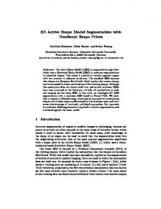
Fig. 1. Sequence of images of a rotating cube (3 samples). Features are the visible vertices. The frontal view of the middle image is degenerate. Bottom picture shows the reconstruction with a rank-based algorithm vs. ground-truth and our algorithm

well as in [8], where authors suggest adding a normalization step between the two factors updates. The Guerreiro and Aguiar approach [6] is similar to Aanaes et al [1], since both algorithms, at each iteration, project the data in a rank-4 subspace. The convergence of the referred methods is initially good but it is very susceptible to flatlining. Recently, Buchanan&Fitzgibbon [2] presented a Newton method to improve convergence, and it is today one of the most accurate and robust rankconstrained algorithms. It is important to note that all alternation algorithms use a` priori knowledge of the rank measurement matrix (in this case rank 4) to estimate the completed matrix. However, the rank constraint is not enough to obtain a correct estimate when there are images in the sequence where the 3D points of the known projections belongs to 1D or 2D subspaces. Errors happen because the optimization problem (1) has infinite minimae. Some works try to solve this ambiguity with more a` priori information. In [17], the planar surfaces of the object are known and due to this they impose these constraints to the object’s shape. Another approach considers a smooth camera trajectory [7,19]. If the missing data matrix D is a block-diagonal matrix, we can find the best model (planar or non-planar) to explain each part of the object [11]. But all these strategies can not be used to solve the problem presented in this paper, because we want to recover the 3D shape of an unknown object, without any constraints in the camera trajectory and in missing data pattern. We will show that this objective can be attained by solving problem (1) but constraining camera motion to comply with the rigidity constraints. To obtain this result, an intermediate step is required, leading to a new rigid factorization algorithm. To illustrate the relevance of the problem, consider the simple synthetic example depicted in figure 1. In this case, the considered object is a cube and feature points are its vertices. We 3

generated an artificial sequence of 10 images of a rotating cube. One of the images is a frontal view where visible features belong the one single face of the cube. The bottom graph of figure 1 shows the resulting shape (in red), after completing the missing vertices with one of the state-of-the-art algorithm. The green cube is the result of our algorithm totally coincident with ground truth (no noise). Note that the completed observation matrix was rank 4. In sum, to our knowledge, the current state-of-the-art algorithms in structure from motion with missing data cannot cope with one single degenerate frame in the sequence.

2 Rigid Factorization In this section we will introduce a new factorization algorithm that computes shape and motion under scaled orthography in one single optimization step, and imposing the correct camera model upfront. In other words besides the rank, the correct motion structure is introduced in the factorization process as a constraint. We will show that this constraint is unavoidable if the known data is degenerate. The affine factorization of Tomasi-Kanade does not provide the correct answer. Assume for now that there are no missing points on the data, and that the known data matrix Z is given by Z=W

(1)

where W is called the data matrix. If one object is represented by P points view in F frames, this matrix is composed by stacking the projections of the object’s points in all images, such as ⎡

1 ⎢ u1

W=

⎢ ⎢ 1 ⎢ v1 ⎢ ⎢ . ⎢ .. ⎢ ⎢ ⎢ 1 ⎢u ⎢ F ⎣

⎤

...

uP1 ⎥

... .. .

v1P ⎥ ⎥ .. ⎥ . ⎥ ⎥

...

⎥ ⎥

(2)

⎥ ⎥ uPF ⎥ ⎥ ⎦

vF1 . . . vFP

where upf and vfp are the p point projection in the frame f . Considering the scaledorthographic camera model, (2) can be factorized as Z = MS + tT 1

(3) 4



T

where M[2F ×3] is the motion matrix, S[3×P ] the shape matrix and t = t1u t1v ...tFu tFv the translation vector. The motion matrix is composed by independent matrices: ⎡

M=

⎤

⎢ M1 ⎥ ⎢ ⎥ ⎢ .. ⎥ ⎢ . ⎥ ⎢ ⎥ ⎣ ⎦

MF

Each matrix Mf (also called the motion matrix in frame f ) is composed by the two perpendicular vectors ⎡

⎤f

⎡ ⎤

f ⎢ ix iy iz ⎥ ⎢i ⎥ Mf = ⎣ ⎦ =⎣ ⎦ jx jy jz jf

(4)

It is important to refer that the vectors if and jf are not orthonormal vectors, as usual, but perpendicular with the same norm (the scale factor). Since we are estimating the model’s parameters without missing data, considering that the shape coordinate system is placed in the shape’s centroid, the translation vector has a closed-form solution, t=

1 P



i

Z1i . . .

1 P



 i

(5)

Z[2f,i]

Replacing it in (3) we obtain the so called centered data matrix Zc = MS

(6)

In the scaled orthographic model (the considered model for the data), there are no constraints for S. Instead M should verify the following motion constraints if if = α f jf jf = αf if jf = 0 ∀f ∈ {1, ..., P }

(7) (8) (9)

Unlike the Tomasi-Kanade algorithm [20], the αf parameter (7,8) allows to recover the object’s shape using images with different scales [13]. To satisfy the last specification, the Tomasi-Kanade algorithm’s extension is presented in [23] and the problem is formulated as a Least Squares (LS) problem. Due to this reason, in 5

the noisy data case, the obtained solution does not satisfy exactly these constraints (7,8,9).

2.1 Imposing Rigid Motion Constraints To make the estimation of the missing data possible (presented in section 3), the motion constraints must be satisfied. To do this, we reformulate the optimization problem and propose an iterative algorithm to solve it. The main idea is to find a factorization of Zc (6), such that, M satisfies the orthogonality constraints (7,8,9). So, the usual unconstrained optimization problem [20] is replaced by the following one  S)  ∗ = arg min (M,   M, S

Problem 2

s.t.



f

 S||  2 ||(Zc )f − M f F T

M  = α1 I M 1 1 2×2 .. . T

M  = αF I M F F 2x2 f + α ∈ R , ∀f

 in the The natural way of solving Problem 2 is to search for the motion matrix M motion manifold, defined by the constraints problem above. However, this is still a very hard problem.

 k−1 M k M

R

Fig. 2. Point R is projected in the motion manifold

Instead we propose an iterative algorithm in R2F ×P where the solution found in each iteration (for the optimization problem without constraints) is projected in the motion manifold (figure 2.1). Algorithm 1 is as a version of the power method where in each iteration a motion matrix is calculated (step 2) independently. The procedure of step 2 projects the left factor of Zc onto the manifold of motion matrices (matrices with pairwise orthogonal rows). This projection has a similar derivation to the Procrustes problem [4]. Specifically, we seek the matrix with pairwise orthogonal rows (not orthonormal) which is closest to the left factor of Zc , that is: 6

Algorithm 1 Rigid Factorization 1. Initializations: (factorize Zc using any factorization (e.g. SVD) 0 = B  0 = A, S Zc = AB, R = A, M k=1 2. Project R into the manifold of motion matrices k = arg min  ||R − X ||2 M X f f F f T s. t. Xf Xf = αf I2x2 ∀f α ∈ R+ +

+

k = M k Z , k - Moore-Penrose pseudoinverse 3. S M c + 4. R = Zc S k  −M  5. Verify if ||M k k−1 || < . If not, go to step 2 and k = k + 1.  =M  and S  =S  6. M k k

k = arg min ||R − X||2 = M F X

= arg min X

 f

||Rf −

s. t.Xf XTf = αf I2x2

⎡ ⎤ ⎡ ⎤2     R ⎢ 1 ⎥ ⎢ X1 ⎥ ⎢ ⎥ ⎢ ⎥ ⎢ .. ⎥ ⎢ .. ⎥ ⎢ . ⎥ − ⎢ . ⎥ ⎢ ⎥ ⎢ ⎥ ⎣ ⎦ ⎣ ⎦  XF   RF

F

Xf ||2F

(10)

∀f, α ∈ R+ ⎡

⎤

⎢σ1

k = α U V T , where R = U M f f f f f ⎣ f

0⎥

0 σ2

⎦ VfT

and αf = (σ1 + σ2 )/2

Even though step 2 is solved F times in each iteration, the computational cost is irrelevant because, as (10) shows, it has closed-form solution and is unique (details in Appendix B). In step 3, the estimate of the object’s shape is given by a LS solution. It is important to refer that matrix Rk , used in step 2 and calculated in step 4, is not  to an algorithm’s output, but an auxiliary matrix. This is used to adapt matrix S k  Mk . In terms of complexity, we need to compute two pseudo-inverses and a set of eigen vectors in closed-form (in R3 ). 7

3 Estimating Shape With Missing Data To represent the missing data, we introduce matrix D. Elements D[2∗i−1,j] and D[2∗i,j] of this matrix are 1 if point j is known in frame i and 0 otherwise. Note that if point p’s projection in frame f is unknown, element D[2∗(p−1),f ] and D[2∗p,f ] are 0 by default, but can take some value in R. Due to missing data, the equations presented in section 2 are not valid here. In this view, (3) is replaced by Z=WD

(11)

According to (11) and the orthographic camera model, we have Z = (MS + tT )  D

(12)

In this section, t can not be calculated as in (5) because this expression requires that all data are known. If one point, say p, is known in all frames, the translation vector is computed as

tT = −Z [0 . . . 0 1 0 . . . 0]T = − z1p . . . z[2f,p]       p−1



(13)

P −p

and all measurements are registered to this point. If not this vector is another parameter to estimate.

3.1 Using the rank constraint The rank constraint can be used to calculate the unknown values of Z. This fact is true because, by checking the model (12) and the dimensions of M and S, we can easily conclude that Z has at most rank 4. In this case, we want to find a rank 4 matrix with the known values of Z. Mathematically, this problem corresponds to solve the following optimization problem 

Problem 3



   ∗ = arg min  W − W   D2 (W)  W

s.t.

 W

F

∈ S4

where S4 is the space of matrices with rank equal to 4. This approach allows us to obtain the correct solution for the missing data in case 8

Fig. 3. Features in frame f : the known points in frame f are represented by red circles and the unknown points by green stars

• the object is a full 3D object • the known points of each of the image stream are not coplanar. The solution is not the correct one if it exists, at least, one image where the known points are in the same 1D or 2D subspace (degenerate images). This happens because problem 3 has infinite many solutions, that is, the value of the cost function  is minimum for different values of W. To verify this fact, consider that the translation vector was computed and, consequently we know the centered matrix Zc , given by Zc = MS  D where Zc ∈ S3 . Suppose that the first m points belong to a 2D flat surface and the known points of the image f are these points, precisely (see fig. 3). The object’s shape is known and we can calculate a matrix A such that the plane z = 0 contains the first m points. ⎡

⎢(Zc )[2f −1,1] ⎣ 

⎤

... (Zc )[2f −1,m] ?...?⎥

(Zc )[2f,1] ... (Zc )[2f,m] 

⎡

A

−1

⎢ 11 ⎢ ⎢ ⎢S21 ⎢ ⎣ 

...

 S

1m

 S

[1,m+1]

⎤

a b c⎥ =⎢ ⎣ ⎦A ?...? def ⎦





f W  S

⎡

 ...S

⎤



f M

(14)



1P ⎥

⎥

   ⎥ ... S 2m S[2,m+1] ...S2P ⎥ ⎥

  0 ... 0 S [3,m+1] ...S3P   S

⎦ 

This particular parametrization just makes completely clear that the submatrix of the first m columns of S is singular (the planar surface). Equation (14) is equivalent to the equation system given by 9

⎧ ⎪ ⎪ (Zc )[2f −1,1] ⎪ ⎪ ⎪ ⎪ ⎪ (Z ) ⎪ ⎪ ⎨ c [2f,1]

..

= aS11 + bS21 = dS11 + eS21 . = ..

(Zc )[2f,m]

= aS1m + bS2m = dS1m + eS2m

. ⎪ ⎪ ⎪ ⎪ ⎪ (Zc )[2f −1,m] ⎪ ⎪ ⎪ ⎪ ⎩

(15)

In the system of equations (15) we can clearly verify that Problem 3 has two degrees of freedom, variables c and f . Then, the unknown image points projection in frame f have not two solutions, but infinite. This fact does not allow us to recover the original motion and shape matrix because the method can add an error to the known points’ projections in this frame. In other words, there can be a large error in the image position (due an arbitrary c and f parameters) and yet the (completed) observation matrix will be rank 4 and not conformal with the orthographic camera model. In real situations with noise and other distortions these estimated projections can be quite far from reality. If, as it is common in real situations, there are large sets of degenerate images and the total error can be significant. In summary, regardless of the algorithm we may use to fill the missing values, there are two free variables which will distort the track matrix and thus distort the shape and the motion.

3.2 Imposing the orthogonality constraints

Considering the orthographic camera model to explain the data, as section 3.1 shows, the rank constraint is not enough to estimate the missing data. The problem formulation must be corrected by including the motion constraints, leading to the following optimization problem   f  Wf

 S)  ∗ = arg min (M,  M S

Problem 4

s.t.



2 

 S   −M f + tf 1[2,P ]  D

T

M  = α1 I M 1 1 .. .

F

T

M  = αF I M F F f α ∈ R+ , ∀f

In this case, variables c and f , instead of an infinite number of solutions, have the two expected solutions (see fig. 4), given by 10

3

2 ← Image 1

Z

1

0

−1 ← Image 2 −2

0

0.5

1

1.5

2

X

2

2

1.5

1.5

1

1

0.5

0.5

Y

Y

−3

0

0

−0.5

−0.5

−1

0

0.5

1

1.5

X

2

2.5

3

−1

0

0.5

2.5

1

1.5

X

3

2

2.5

3

Fig. 4. Two solutions: the known points in frame f are represented by red circles and the unknown points by green circles. Bottom Left - 2D projections in image 1. Bottom Right 2D projections in image 2. 





 1 c=± −a2 − b2 + d2 + e2 + gh 2 



(16)



 1 2 2 2 2 f =∓ a + b − d − e + gh 2

(17)

where g = d2 + 2db + b2 + e2 − 2ea + a2 and h = d2 − 2db + b2 + e2 + 2ea + a2 (details in Appendix A). The two solutions correspond to the correct one, and the reflection of the camera over the plane (shape). This reflection produces the same image (it is intrinsic to orthography). Even though motion can be ”reflected” the computed shape will always be correct, up to the ambiguity of an orthogonal transformation, inherent to the orthographic model. This means both that the Motion and Shape matrix fit the known data and also that the Motion matrix satisfies the orthogonality constraints. Note that the case of known data over a line (the known part of shape is rank 1) there will be infinite solutions for motion too. However, this will not affect the 11

Algorithm 2 Rigid Factorization with Missing Data  = Z, k = 0 1. Initializations: Z 0 2.Estimate translation (centroid). 

   ... 1  Z  tk = P1 i Z 1ik i [2f,i] k (13) P

 =Z  − Z tk Remove translation ck k k =k+1  and S  Using Rigid Factorization 3. Estimate M k k 4. Update data matrix  S   ¯ Zk = (M Z D k k + tk−1 1[2F,P ] )  D +    





Known data Missing data estimate ¯ - 2’s complement of D i.e. D ¯ = 1[2F,P ] − D D   5. Verify if ||Zk − Zk−1 || < . If not verify go to step 2 and k = k + 1.

shape either (orthography is valid). Then, to compute the structure from motion it is proposed the iterative Algorithm 2. In step 1 (Initialization), the entries missing in data matrix Z are initialized with random values in the range of the known entries. In step 3, we use an algorithm whose solution verifies (7,8,9) such as the algorithm described previously(Algorithm 1). It is important to note that the translation vector is not estimated (step 2) if at least one point is known in all images (13). As the proposed algorithm is iterative, convergence is an essential topic while evaluating its performance. Due to this, we did some synthetic experiments to illustrate the algorithm’s behavior in different situations. The obtained results are presented in the end of the next section. In summary, the optimization strategy proposed here is similar to the power factorization [8], but, in our case the rigidity constraints are imposed in each step. In summary, the optimization strategy proposed here is based on a EM view of the missing data problem such as [5,6]. In formal terms, our method is quite similar to the power factorization [8] since the first steps are the same. However, in this case, the rigidity constraints are imposed in each step (adding a projection on the motion manifold) guaranteeing that we obtain one motion matrix exactly and thus solving the degenerate case. 12

4 Experiments

4.1 Hotel Experiment Benchmark tests were performed against the state-of-the-art, using Buchanan and Fitzgibbon’s matlab code 1 . To prevent a full match between the data and our model we only used real data. We modified the known hotel sequence 2 , selecting all 106 feature points and 18 equally spaced frames from the total of 180. A random pattern of missing features was generated with only 14% missing features. Two of those frames were artificially made degenerate with only 24 features visible, all lying on a planar surface (the rightmost wall of the hotel, shown in figure 5 top right). Since there is no ground-truth, we used the object’s shape computed using TomasiKanade’s factorization method with full observation matrix (no missing data), as the reference shape (figure 5 middle). In figure 6 we show the performance of our (rigid factorization) algorithm against 4 state-of-the-art methods: BF-Buchanan&Fitzgibbon’s Damped Newton method[2], PF- power factorization [8,22] 3 , GA- Guerreiro&Aguiar EM (alternate) algorithm [6],Aanaes- Aanaes et al [1]. To avoid graphical clutter, in the top plot of figure 6 we show the reconstruction of two methods (GA and BF), the ”ground-truth”(TK) and our method (RF). Note that an euclidian upgrade was performed to all matrix completion algorithms to obtain a 3D reconstruction. The figure was generated from a top view so that the 3 planes of the hotel walls can be perceived clearly. Recall that GA and BF are quite different in nature (an alternate algorithm vs. a Newton algorithm). Since both methods seek the best rank 4 matrix they reach similar solutions, both inadequate. As expected by enforcing rigidity constraints the reconstruction is quite close to the reference. All other methods behaved in much the same way, and this is reflected in the error plot shown in the bottom graph of figure 6. Here, each  bar represents the percentage of shape error ( |Sˆi −Sitk |)/(max(S tk ) −min(S tk )), where Sˆi is the shape estimate for point i and Sitk is the reference shape for that point. Of course the absolute value of the error depends on the particular shape, but the relevant aspect is that all other methods obtain estimates that are at least one order of magnitude above our method, and this happens with only 14% of data missing. The large errors obtained by rank-based methods is because the degeneracy is not addressed explicitly. Since they assume data modeled as W = AB they try to estimate independently all values of A and B. In this way, they are estimating values c and f in equation(14), when these variables should be assigned by the orthogonality constraint (17). 1

This package contains several high performance methods and was made generously available in www.robots.ox.ac.uk/˜abm 2 http://vasc.ri.cmu.edu/idb/html/motion/index.html 3 Though the first reference introduced the method, the code cites the second

13

200 150 100 50

100 0

0 −100

−50 −100 −150 −200

−200

−100 0 100

Image

0 10 0

20

40

60 Feature

80

100

Fig. 5. Up Left -Feature tracks of the sequence. Up Right - features in the degenerate frames. Middle - The reference 3D shape, computed with Tomasi-Kanade’s factorization. Bottom - Pattern of missing points. First 2 images are degenerate

4.2 Dinosaur Experiment In the second experiment with real data, the proposed algorithm was tested with other well-known sequence - the dinosaur sequence 4 (figure 7). In the opposite way to the hotel sequence, this one, which is composed by 36 images, does not 4

www.robots.ox.ac.uk/˜abm

14

TK BF GA RF

100 0 −100

200 0 −200

−300

−200

−100

0

100

200

25

Shape error (%)

20

15

10

5

0

Aanaes

BF

GA

RF

PF

Fig. 6. The top figure compares several methods by showing a top view of the hotel’s 3D shape. Besides the reference shape (TK), we show the proposed method (RF) and two other (BF and GA). The graph in the bottom figure plots the relative error of several methods showing that none of the rank-based methods (Aanaes, BF, GA and PF) can compute shape adequately

contain any image with degenerate data and the measurement matrix is sparse with only 28% of known data (see figure 7). The dinosaur sequence was used to evaluate the the performance of our ”rigid factorization” algorithm with highly sparse data sets. Since the complete matrix is not available, we will compare our algorithm against the most accurate algorithm for this type of problem. To our knowledge, the Damped Newton algorithm of Buchanan&Fitzgibbon [2] produces the least reconstruction error (it is optimal 15

Image

0 20 0

50

100

150 Feature

200

250

300

Fig. 7. Up - Two images of the sequence Bottom - Pattern of missing points

for this criterion). The error measure is the √ root mean square error of the known data, that is  = ||(W − MS)  D||F / N1 . Here N1 represents the number of observed points. In figure 8 we show the position of the reprojection of the visible points (wi = mi ∗ S) for one particular image of the sequence. The total rms error for the whole sequence is 1.3705, though some points have a considerably high deviation. These points are shown in the right picture of figure 8. As both pictures show, except for peripherical areas, the majority of points are estimated with a reasonably low error. The fact that our algorithm exhibits larger error is is an expected result due to the extra constraints imposed on the fitting model. Since we impose rigidity, there are less degrees of freedom to adjust to the error. For a qualitative evaluation, figure 9 shows the dinosaur’s shape. Original B&F RF

Original B&F RF

Fig. 8. The left picture shows the original image points and their re-projections both for the proposed algorithm and the state of the art. The RMS error is 1.3705 pixels, higher than the ”best” value of 1.0847. Maximum error was 21 pixels, as the right figure shows.

16

−300 −200 −100 0 100 200 300

300

200

100

−200 −300 0 −100

100 0 −100

Fig. 9. The dinosaur’s 3D shape

4.3 Full reconstruction with largely scaled images In the third experiment, we present a real life example using the rigid factorization with missing data. The aim is to produce a 3D reconstruction of one building from a set of uncalibrated images. We searched on Google for images depicting the building (search ”casa da musica”) from a quite diverse set of viewpoints. The image scale is also quite diverse, since there are images taken from a pedestrian capturing one window together with far off aerial views from an airplane. Resolution ranged from 3 Megapixel to a 60 Kilopixel and perspective effects were quite large in some of them. Image features were tracked by hand and were basically the vertices of the building and windows’ corners. In figure 10 we show some of the 19 images with the features superimosed. Features are missing due to occlusion but also because we did not insert all visible points. Close up views with a large depth range produce strong perspective, therefore we just inserted points that were in a small depth range compared to the distance to the camera. Even though it favors the camera model adequacy it generates high volumes of (possibly degenerate) missing data. A triangulation was computed to convey the shape in a more natural way. The blue surfaces are windows. As figure 10 shows, the reconstruction is quite faithful. However perspective effects are noticeable, specially in the large front window. Nevertheless, in our opinion, this is quite a hard set of images to any 3D reconstruction algorithm and remember that no prior knowledge is used. For more precise applications this can be a good starting point for perspective factorization algorithms such as [9,18].

4.4 An urban modeling example In the last experiment, the scenario is also 3D building reconstruction (figure 11). But, in this case, the goal is very hard to achieve due to the few images available and to the high percentage of missing data. In this case the object is composed of 21 features and there are 7 images available (figure 11 - bottom). As the pattern of missing data in figure 11-bottom shows, the missing data is almost 60% and image 4 (bottom-right image in figure 11-top) and image 5 are degenerate. 17

Fig. 10. Reconstruction of a famous Rem Koolhaas ”piecewise planar” building. Blue dots represent feature location. Third row shows reconstruction with the proposed method

Another relevant fact in this experiment is that features 7 and 8 only appear twice in the whole sequence (the minimum number) and feature 21 only 3 times. Despite the difficulties mentioned above, we obtain a quite good result (figure 12). In the top images of figure 12, we can clearly see that the feature 8 is the only one in a wrong 3D position: it is not aligned with features 2 and 5 as it was expected (remember that feature point 8 appears 2 times only). This artifact disappears in the bottom images because the presented 3D reconstruction only uses the faces’ corners of the building. Through this example, we can say that the presented method is a very useful tool to obtaining 3D reconstructions from few images of the considered object and a large percentage of missing data. 4.5 Convergence To analyze the algorithm’s performance, several synthetic experiments were done. Convergence was evaluated as a function of the total number of points and the number of visible points. The test object was composed of 3 faces of a cube and the number of features ranged from 12 (4 in each face) to 111 features (37 in each face). In each experiment, a total of 21 images were generated and 15 of them were degenerate, that is, the visible points in these images belonged to 1 face only. The 18

0

Image

2 4 6 8

0

5

10 Feature

15

20

Fig. 11. Up - A typical example of urban modeling. From left-right and up-bottom, images #7-2-1-4 of the sequence. Top-left image has feature number superimposed. Bottom Pattern of missing points:X-axis represent point # and Y-axis the image #

missing data in the remaining 6 (non-degenerate) images was set to 30%. Figure 13 plots graphs of the ratio and speed of convergence. One hundred random experiments were made for each pair of parameters (#points, #visible points). Even though the number of degenerate images is significant (71% in this case), the convergence rate is not directly influenced by the percentage of missing data. Instead, 19

7

4

−200

−300

−200 17

16

10

3

−100

2

1 200

1

8

150

21

5 20

2

50

18

12

13

3

−100 −100

0

200

17

8

200

14

15

20

200 21 −100 0 100 200

7

11 100

9

0

16

10 −200

100

4

0 −50

0 19

18

13

5

19

15

14

6

12

6

9

100

−300

300

200

100 11

0

−100

300

−200

Fig. 12. Top graphs show the 3D point reconstruction (shape). In the bottom figure, the image is mapped on a piecewise planar model, created with the corners of each plane.

it is affected by the number of known projections in degenerate images. To obtain good estimations, we must know at least 8 points per each degenerate image. In other words rates of convergence above 97% are attained, provided that at least 8 points are visible, regardless of the number of missing points. In the same line of the previous result, the convergence’s velocity changes in accordance to the known projections in degenerate frames: the new algorithm is faster when more projections are known (see fig. 13 Bottom). The graphs of figure 14 illustrate the algorithm’s behavior with noise and the number of visible points in degenerate images. Note that the percentage of noise is related to the values of the object’s projections in each image, e.g. if the object’s size in image f is 500 × 500 pixels and noise is 10%, the projection’s error will be 50 pixels. In this experiment, the number of points was chosen such that a high convergence rate is achieved: the object (the same 3 faces of a cube) has 39 features (13 in each face). Thus, the number of known projections in degenerate images (15 in 21 also) is between 8 and 13. The figure of merit to the algorithm’s evaluation is shape error. Observing figure 14, we straightforwardly conclude that performance (error) depends on noise power. These results are compared with the reference shape, computed by TK factorization with full matrix. We can verify that the error shape is proportional to that of the reference shape. In summary, the relevant conclusion here is that the proposed algorithm converges ”on average” to the correct shape, when there are at least 8 known points in each degenerate image. 20

100

Convergence (%)

80 60 40 20 0 20 40 60 80 100

5

10

15

20

35

30

25

Viewed points in each degenerate frame

Nº of iterations

8000 6000 20

4000 40 2000

60 5

10

15

80 20

25

30

100 35

Viewed points in each degenerate frame

Fig. 13. Top - Convergence:Zaxis- % of converged trials.Xaxis- Number of visible points in degenerate. Yaxis -Total number of points - Bottom - Zaxis-Number of iterations vs. the same parameters as before

Fig. 14. Shape error as a function of noise and number of visible points

5 Conclusions We have presented an new factorization algorithm that computes the optimal motion shape and scale estimates (scaled orthography) from a feature track matrix. 21

We also introduced an iterative algorithm that produces the same estimates when feature points are missing and the known points are degenerate. To our knowledge no other algorithm can solve this problem. We have presented a solution of the structure from motion problem to the most general and realistic situation.

A Consider the following system of equations ⎧ 2 ⎪ ⎪ ⎨a

+ b2 + c2 d2 + e2 + f 2 ⎪ ⎪ ⎩ ad + be + cf

= α2 = α2 =0

(A.1)

where a, b, c and d are not variables of this problem. Considering only the first two equations, we can write ⎧ ⎨a2

+ b2 + c2 ⎩ad + be + cf

= d2 + e2 + f 2 =0

(A.2)

To obtain c and f , the last equation is solved in order to both variables, ⎧ ⎨c2

+ (a2 + b2 − d2 − e2 ) c − a2 d2 − b2 e2 − 2adbe = 0 ⎩f 2 + (−a2 − b2 + d2 + e2 ) f  − a2 d2 − b2 e2 − 2adbe = 0

(A.3)

To simplify the notation, it is important to note that these 2nd order equations (A.3) were obtained by the following change of variables: c = c2 and f  = f 2 . Due to the similarity between the equations, the following steps aim to calculate c, because f is obtained in the same way. Then, the roots of first equation are 



 1 −a2 − b2 + d2 + e2 ± gh c = 2 

where g = d2 + 2db + b2 + e2 − 2ea + a2 and h = d2 − 2db + b2 + e2 + 2ea + a2 . Because of c = c2 and c ∈ R, c is, necessarily, 0 or a positive value. Due to this we consider the first root. Then, the value of c is given by 22







 1 c=± −a2 − b2 + d2 + e2 + gh 2

(A.4)

Through an analogous way, f is given by 





 1 2 f =∓ a + b2 − d2 − e2 + gh 2

(A.5)

B Considering the optimization problem given by

X∗ = arg minX ||A − X|| s.t. XXT = α2 I T and the Singular Value Decomposition of A and X, this is A = UA ΣA VA and T X = UX ΣX VX , we have





T T   X∗ = arg minX UA ΣA VA − UX ΣX VX

X∗ = arg minX tr



s.t. XXT = α2 I  T T UA ΣA VA − UX ΣX VX



T T UA ΣA VA − UX ΣX VX

T 

s.t. XXT = α2 I As the matrix X∗ is, by definition of the optimization problem, the nearest matrix of A (considering the Frobenius norm), we have UA = UX and VA = VX . If we do not consider the constant term of the cost function and, to simplify the notation, we replace UA and VA by U and V, respectively, we arrive to Σ∗X = arg minΣX −2tr s.t.





UΣA VT

UΣX VT





UΣX VT

UΣX VT

T

T 

+ tr



UΣX VT



UΣX VT

= α2 I

Imposing the constraint into the cost function, we have the following optimization problem without constraints 23

T 

∗

α = arg minα −2tr



UΣA V

T



UαIV

T

T 

+ tr (α2 I)

  α = arg minα −2αtr UΣA VT VUT + α2 tr (I)  ∗ α = arg minα −2αtr (ΣA ) + α2 tr (I) ⎛⎡ ⎤⎞ 

∗

⎢λ1 0 ⎥⎟ α∗ = arg minα −2αtr ⎜ ⎝⎣ ⎦⎠ + α2 tr (I) 0 λ2  ∗ α = arg minα −2α (λ1 + λ2 ) + 2α2

where λ1 and λ2 are the singular values of A. To find a maximum of the cost function (now called by f (α)), we calculate the stationary points of this function. These points are given by ∂f =0 ∂α

(B.1)

Solving (B.1) we obtain α∗ =

λ1 + λ2 2

(B.2)

As we wished, the found solution (B.2) is a global minima of f (α) because ∂2f = 2 > 0, ∀α∈R ∂α2

(B.3)

Then, X∗ is given by ⎡ ⎢α

X∗ = U ⎣

∗

⎤

0⎥

0 α

∗

⎦V

T

(B.4)

References [1] H. Aanaes, R. Fisker, K. Astrom, and J. M. Carstensen. Robust factorization. IEEE Trans. Pattern Anal. Mach. Intell., 24(9):1215–1225, 2002.

24

[2] A. Buchanan and A. Fitzgibbon. Damped newton algorithms for matrix factorization with missing data. In Proceedings of the IEEE Conference on Computer Vision and Pattern Recognition, volume 2, pages 316–322, 2005. [3] S. Christy and R. Horaud. Euclidean shape and motion from multiple perspective views by affine iterations. IEEE Trans. Pattern Anal. Mach. Intell., 18(11):1098–1104, November 1996. [4] G. Golub and V. Loan. Matrix computations. [5] R. Guerreiro and P. Aguiar. Factorization with missing data for 3d structure recovery. IEEE Multimedia Signal Processing Workshop September 2002, St. Thomas, USA, 2002. [6] R. Guerreiro and P. Aguiar. Estimation of rank deficient matrices from partial observations: Two-step iterative algorithms. Proc. Conf. Energy Minimization Methods in Computer Vision and Pattern Recognition., 2003. [7] N. Guilbert, A. Bartoli, and A. Heyden. Affine approximation for direct batch recovery of euclidean motion from sparse data. Int. Journal of Computer Vision, 69(3):317–333, September 2006. [8] R. Hartley and F. Schaffalitzky. Powerfactorization: 3d reconstruction with missing or uncertain data. In Australia-Japan Advanced Workshop on Computer Vision, 2003. [9] A. Heyden, R. Berthilsson, and G. Sparr. An iterative factorization method for projective structure and motion from image sequences. Image Vision Comput., 17(13):981–991, 1999. [10] D. Jacobs. Linear fitting with missing data: Applications to structure-from-motion and to characterizing intensity images. In IEEE International Conference on Computer Vision, pages 206–212, 1997. [11] K. Kanatani. Geometric information criterion for model selection. Int. J. Computer Vision, 26(3):171–189, 1998. [12] D. Martinec and T. Pajdla. 3d reconstruction by fitting low-rank matrices with missing data. CVPR, 2005. [13] C. Poelman and T. Kanade. A paraperspective factorization method for shape and motion recovery. IEEE Trans. Pattern Anal. Mach. Intell., 19(3):206–218, 1997. [14] I. Reid and D. Murray. Active tracking of foveated feature clusters using affine structure. Int. Journal of Computer Vision, 18(1):41–60, 1996. [15] S. Roweis. Em algorithms for pca and spca. Proceedings NIPS, 10:626–632, 1997. [16] H. Shum, K. Ikeuchi, and R. Reddy. Principal component analysis with missing data and its application to polyhedral object modeling. IEEE Trans. Pattern Anal. Mach. Intell., 9(2):137–154, 1995. [17] G. Sparr. Euclidean and affine structure/motion for uncalibrated cameras from affine shape and subsidiary information. In SMILE Workshop on Structure from Multiple Images, Freiburg, 1998.

25

[18] P. Sturm and B. Triggs. A factorization based algorithm for multi-image projective structure and motion, 1996. [19] J.-P. Tardif, A. Bartoli, M. Trudeau, N. Guilbert, and S. Roy. Algorithms for batch matrix factorization with application to structure-from-motion. Proceedings of the IEEE Conference on Computer Vision and Pattern Recognition, June 2007. [20] C. Tomasi and T. Kanade. Shape and motion from image stream under orthography: a factorization method. Int. Journal of Computer Vision, 9(2):137–154, 1992. [21] B. Triggs. Linear projective reconstruction from matching tensors. Image and Vision Computing, 15(8):617–625, 1997. [22] R. Vidal and R. Hartley. Motion segmentation with missing data using powerfactorization and gpca. Proceedings CVPR, 2:310–316, 2004. [23] D. Weinshall and C. Tomasi. Linear and incremental acquisition of invariant shape models from image sequences. IEEE Trans. Pattern Anal. Mach. Intell., 17(5):512– 517, 1995. [24] T. Wiberg. Computation of principal components when data are missing. Proceedings Symposium of Comp. Stat., pages 229–326, 1976.

26