To all my friends here in Kingston and British Colombia (BC), who have made ..... PDF. Probability Density Function. PEP. Pairwise Error Probability. PSK ...... [63] Y. Mei, Y. Hua, A. Swami, and B. Daneshrad, âCombating synchronization.
ESTIMATION AND EFFECTS OF IMPERFECT SYSTEM PARAMETERS ON THE PERFORMANCE OF MULTI-RELAY COOPERATIVE COMMUNICATIONS SYSTEMS
by
Mehrpouyan, Hani
A thesis submitted to the Department of Electrical and Computer Engineering in conformity with the requirements for the degree of Doctor of Philosophy
Queen’s University Kingston, Ontario, Canada July 2010
c Copyright ⃝Hani Mehrpouyan, 2010
Abstract
To date the majority of research in the area of cooperative communications focuses on maximizing throughput and reliability while assuming perfect channel state information (CSI) and synchronization. This thesis, seeks to address performance enhancement and system parameter estimation in cooperative networks while relaxing these idealized assumptions. In Chapter 3 the thesis mainly focuses on training-based channel estimation in multi-relay cooperative networks. Channel estimators that are capable of determining the overall channel gains from source to destination antennas are derived. Next, a new low feedback and low complexity scheme is proposed that allows for the coherent combining of signals from multiple relays. Numerical and simulation results show that the combination of the proposed channel estimators and optimization algorithm result in significant performance gains. As communication systems are greatly affected by synchronization parameters, in Chapter 4 the thesis quantitatively analyzes the effects of timing and frequency offset on the performance of communications systems. The modified Cramer-Rao lower bound (MCRLB) undergoing functional transformation, is derived and applied to determine lower bounds on the estimation of signal pulse amplitude and signal-to-noise ratio (SNR) due to timing offset and frequency offset, respectively. i
In addition, it is shown that estimation of timing and frequency offset can be decoupled in most practical settings. The distributed nature of cooperative relay networks may result in multiple timing and frequency offsets. Chapters 5 and 6 address multiple timing and frequency offset estimation using periodically inserted training sequences in cooperative networks with maximum frequency reuse, i.e., space-division multiple access (SDMA) networks. New closed-form expressions for the Cramer-Rao lower bound (CRLB) for multiple timing and multiple frequency offset estimation for different cooperative protocols are derived. The CRLBs are then applied in a novel way to formulate training sequence design guidelines and determine the effect of network protocol and topology on synchronization parameter estimation. Next, computationally efficient estimators are proposed. Numerical results show that the proposed estimators outperform existing algorithms and reach or approach the CRLB at mid-to-high SNR. When applied to system compensation, simulation results show that application of the proposed estimators allow for synchronized cooperation amongst the nodes within the network.
ii
Coauthors
List of publications as a result of this thesis’s contributions:
Chapter 2: Hani Mehrpouyan and Steven D. Blostein, “ARMA Synthesis of the Fading Channels,” IEEE Transactions on Wireless Commun., vol. 7, no. 8, Feb. 2008. Hani Mehrpouyan and Steven D. Blostein, “ARMA Synthesis of Fading Channels: an Application to the Generation of Dynamic MIMO Channels,” IEEE Globecom, Nov. 2007. Hani Mehrpouyan, Steven D. Blostein, E. C. Y. Tam “Random Antenna Selection and Antenna Swapping Combined with OSTBCs,” IEEE ISSSE, Aug. 2007. Chapter 3: Hani Mehrpouyan, Yi Zheng, and Steven D. Blostein, “On Channel Estimation and Capacity Enhancement for Multi-Relay MIMO Cooperative Networks,” Submitted to IEEE Trans. on Wireless Commun., second round of review, March, 2010. Yi Zheng, Hani Mehrpouyan, and Steven D. Blostein, “Application of Phase Shift in Coherent Multi-Relay MIMO Communications,” IEEE Inter. Conf. on Commun., Jun. 2009.
iii
Chapter 5: Hani Mehrpouyan and Steven D. Blostein, “Estimation, Training, and Effect of Timing Offsets in Distributed Cooperative Networks,” Submitted to IEEE Globecom, March 2010. Hani Mehrpouyan and Steven D. Blostein, “Synchronization in Distributed Cooperative Network: Bounds and Algorithms for Estimation of Multiple Timing Offsets,” Submitted to IEEE Trans. on Signal Proc., Feb. 2010. Hani Mehrpouyan and Steven D. Blostein, “Bounds on Timing Jitter Estimation in Cooperative Networks,” QBSC, May 2010. Chapter 6: Hani Mehrpouyan, and Steven D. Blostein, “Bounds and Algorithms for Multiple Frequency Offset Estimation in Cooperative Networks,” Submitted to IEEE Trans. on Wireless Commun., June 2010. Hani Mehrpouyan and Steven D. Blostein, “Frequency Synchronization in 3Terminal and 2-Hop Cooperative Networks,” Submitted to IEEE Globecom, March 2010. Hani Mehrpouyan and Steven D. Blostein, “Synchronization in Cooperative Networks: Estimation of Multiple Carrier Frequency Offsets,” IEEE Inter. Conf. on Commun., May 2010.
iv
Dedication
To Sonia and my parents Golali and Fatemeh, who have supported me every step of the way and sacrificed so much for me.
v
Acknowledgments
I have had the honor and pleasure of working with Dr. Steven D. Blostein throughout my Masters and Ph.D. years at Queen’s University. Through Dr. Blostein’s help and guidance, we have been able to address many challenging topics in the area of wireless communications and advance the research in this discipline. I would like to thank Dr. Blostein for not just being a supervisor but also for being a great mentor and friend through the ups and downs of this challenging but rewarding program. I look forward to continuing my collaboration with him after the completion of my Ph.D. degree. I would also like thank my beloved fiance, Sonia Perizzolo for being by my side throughout the years. My parents, Fatemeh and GolAli for supportingly me unequivocally. Without their help and support I would have never made it this far. My Sister, Hoda for always cheering me up with her beautiful smile from a very young age. I want to thank you all from the bottom of my heart. To all my friends here in Kingston and British Colombia (BC), who have made the past five years a blast. I would like to specially thank Chris Mitchell, and my labmates, Yu, Yi, Minhua, Jinsong, Hassan, Alex, Viet-Anh, and Jason. Finally, I would like to extend my gratitude to the Natural Sciences and Engineering Research Counsel (NSERC), Communications Research Centre (CRC), vi
Defence Research and Development Canada, and Queen’s Graduate Awards for funding my graduate studies during the past five years.
vii
Contents
Abstract
i
Copyright
iii
Dedication
v
Acknowledgments
vi
List of Tables
xiii
List of Figures
xviii
Acronyms
xix
List of Important Symbols Chapter 1
xxii
Introduction
1
1.1
Cooperative Systems for Future Wireless Communications . . . . . .
1
1.2
Motivation and Thesis Overview . . . . . . . . . . . . . . . . . . . . .
3
1.3
Thesis Contributions . . . . . . . . . . . . . . . . . . . . . . . . . . . .
9
Chapter 2 2.1
Background
11
Point-to-Point MIMO Systems . . . . . . . . . . . . . . . . . . . . . . . 11
viii
2.2
Cooperative Systems . . . . . . . . . . . . . . . . . . . . . . . . . . . . 13 2.2.1
Amplify-and-Forward . . . . . . . . . . . . . . . . . . . . . . . 14
2.2.2
Decode-and-Forward . . . . . . . . . . . . . . . . . . . . . . . 15
2.3
Channel Model . . . . . . . . . . . . . . . . . . . . . . . . . . . . . . . 15
2.4
Synchronization Parameters . . . . . . . . . . . . . . . . . . . . . . . . 17 2.4.1
Timing Offset . . . . . . . . . . . . . . . . . . . . . . . . . . . . 18
2.4.2
Carrier Frequency Offset (CFO) . . . . . . . . . . . . . . . . . . 19
2.4.3
Phase Offset . . . . . . . . . . . . . . . . . . . . . . . . . . . . . 22
2.4.4
Cramer-Rao Lower Bound . . . . . . . . . . . . . . . . . . . . . 22
2.4.5
MUSIC Algorithm for Frequency Offset Estimation . . . . . . 23
Chapter 3
Channel Estimation and Capacity Optimization for Cooperative
Networks
27
3.1
Introduction . . . . . . . . . . . . . . . . . . . . . . . . . . . . . . . . . 27
3.2
System Model . . . . . . . . . . . . . . . . . . . . . . . . . . . . . . . . 30
3.3
3.4
3.2.1
Training Interval . . . . . . . . . . . . . . . . . . . . . . . . . . 31
3.2.2
Data Transmission Interval . . . . . . . . . . . . . . . . . . . . 32
Channel Estimation . . . . . . . . . . . . . . . . . . . . . . . . . . . . . 32 3.3.1
Maximum-Likelihood Estimator (MLE) . . . . . . . . . . . . . 34
3.3.2
Least Squares (LS) Estimator . . . . . . . . . . . . . . . . . . . 35
Relaying Scheme . . . . . . . . . . . . . . . . . . . . . . . . . . . . . . 35 3.4.1
Determining the Phase Shift: SISO Cooperative Network . . . 37
3.4.2
Determining the Phase Shift: MIMO Cooperative Network . . 38
3.5
Numerical Results and Discussions . . . . . . . . . . . . . . . . . . . . 39
3.6
Conclusions . . . . . . . . . . . . . . . . . . . . . . . . . . . . . . . . . 46
ix
Chapter 4
Effects of Timing Jitter and Frequency Offset on System Perfor-
mance
47
4.1
Introduction . . . . . . . . . . . . . . . . . . . . . . . . . . . . . . . . . 47
4.2
Modified CRLB . . . . . . . . . . . . . . . . . . . . . . . . . . . . . . . 50
4.3
MCRLB under functional transformation . . . . . . . . . . . . . . . . 53
4.4
Applications of the Functional Transformation of the MCRLB . . . . 54 4.4.1
Effect of Timing offset on the RC, RRC, and FEX Pulses . . . . 55
4.4.2
Effect of Frequency Offset on OFDM Systems . . . . . . . . . . 62
4.5
MCRLB vs. CRLB for Synchronization Parameter Estimation . . . . . 66
4.6
Conclusions . . . . . . . . . . . . . . . . . . . . . . . . . . . . . . . . . 69
Chapter 5
Timing Offset Estimation in Distributed Cooperative Networks 70
5.1
Introduction . . . . . . . . . . . . . . . . . . . . . . . . . . . . . . . . . 70
5.2
System Model . . . . . . . . . . . . . . . . . . . . . . . . . . . . . . . . 74 5.2.1
Training Signal Model at the Relays . . . . . . . . . . . . . . . 76
5.2.2
Training Signal Model at the Destination for DF Relaying Cooperative Networks . . . . . . . . . . . . . . . . . . . . . . . . 78
5.2.3
Training Signal Model at the Destination for AF Relaying Cooperative Networks . . . . . . . . . . . . . . . . . . . . . . . . 79
5.2.4 5.3
5.4
Multiple Timing Offset Estimation in Cooperative Networks . 81
Cramer-Rao Lower Bound . . . . . . . . . . . . . . . . . . . . . . . . . 82 5.3.1
Decode-and-Forward Cooperative Networks . . . . . . . . . . 82
5.3.2
Amplify-and-Forward Cooperative Networks . . . . . . . . . 85
Training Sequence Design . . . . . . . . . . . . . . . . . . . . . . . . . 88 5.4.1
Training Sequence Design for DF Relaying Networks . . . . . 88
5.4.2
Training Sequence Design for AF Relaying Networks . . . . . 91 x
5.5
5.6
5.7
Proposed Timing Offset Estimator . . . . . . . . . . . . . . . . . . . . 91 5.5.1
MLE for Multiple Timing Offset Estimation . . . . . . . . . . . 92
5.5.2
I-MLE for DF Networks . . . . . . . . . . . . . . . . . . . . . . 94
5.5.3
I-GD for DF Networks . . . . . . . . . . . . . . . . . . . . . . . 96
5.5.4
I-MLE and I-GD for AF Networks . . . . . . . . . . . . . . . . 99
5.5.5
Complexity Analysis and Comparison . . . . . . . . . . . . . . 99
Numerical Results and Discussions . . . . . . . . . . . . . . . . . . . . 101 5.6.1
Estimation Performance . . . . . . . . . . . . . . . . . . . . . . 102
5.6.2
Cooperative Network Performance . . . . . . . . . . . . . . . 110
Conclusion . . . . . . . . . . . . . . . . . . . . . . . . . . . . . . . . . . 112
Chapter 6
Carrier Frequency Offset Estimation in Distributed Cooperative
Networks
115
6.1
Introduction . . . . . . . . . . . . . . . . . . . . . . . . . . . . . . . . . 115
6.2
System Model . . . . . . . . . . . . . . . . . . . . . . . . . . . . . . . . 119
6.3
6.4
6.5
6.2.1
Training Signal Model for DF Relaying Cooperative Networks 120
6.2.2
Training Signal Model for AF Relaying Cooperative Networks 122
Cramer-Rao Lower Bound . . . . . . . . . . . . . . . . . . . . . . . . . 124 6.3.1
Decode-and-Forward Cooperative Networks . . . . . . . . . . 124
6.3.2
Amplify-and-Forward Cooperative Networks . . . . . . . . . 127
Proposed CFO Estimators . . . . . . . . . . . . . . . . . . . . . . . . . 129 6.4.1
I-MUSIC for DF Networks . . . . . . . . . . . . . . . . . . . . . 129
6.4.2
I-C-MUSIC for DF Networks . . . . . . . . . . . . . . . . . . . 135
6.4.3
CFO Estimation in AF Networks . . . . . . . . . . . . . . . . . 135
6.4.4
Complexity of I-MUSIC and I-C-MUSIC . . . . . . . . . . . . . 137
Numerical Results and Discussions . . . . . . . . . . . . . . . . . . . . 138 xi
6.6
6.5.1
Estimation Performance . . . . . . . . . . . . . . . . . . . . . . 138
6.5.2
Cooperative Network Performance . . . . . . . . . . . . . . . 144
Conclusion . . . . . . . . . . . . . . . . . . . . . . . . . . . . . . . . . . 147
Chapter 7
Conclusions and Future Work
148
7.1
Conclusions . . . . . . . . . . . . . . . . . . . . . . . . . . . . . . . . . 148
7.2
Future Work . . . . . . . . . . . . . . . . . . . . . . . . . . . . . . . . . 150
Bibliography
153
xii
List of Tables 5.1
I-MLE Timing offset Estimator . . . . . . . . . . . . . . . . . . . . . . 97
5.2
Number of additions and multiplication for MLE-AP, I-MLE, and I-GD ×107 . . . . . . . . . . . . . . . . . . . . . . . . . . . . . . . . . . 101
6.1
Initialization Steps for I-MUSIC and I-C-MUSIC . . . . . . . . . . . . 133
xiii
List of Figures 1.1
MIMO channel with M transmit and N receive antennas. . . . . . . .
1.2
The conventional direct link, two-hop, and relay communications
3
schemes [16]. Note that S, R, and D stand for source, relay, and destination, respectively. . . . . . . . . . . . . . . . . . . . . . . . . . . 1.3
4
Block diagram representing the algorithm executed at the relay under AF and DF protocols. Note that S and D stand for source and destination, respectively. . . . . . . . . . . . . . . . . . . . . . . . . . .
4
2.1
System model for a MIMO cooperative network. . . . . . . . . . . . . 12
2.2
Eye diagram representing the effect of ISI. . . . . . . . . . . . . . . . . 19
2.3
Constellation rotation due to frequency offset. . . . . . . . . . . . . . 20
2.4
SNR loss due to frequency offset, ν for OFDM systems. . . . . . . . . 21
2.5
Maximization in (2.25) versus the normalized frequency for Nl = 16 and SNR= 20. A. The received signal is a combination of 4 signals with ν1 = .1, ν2 = .2, ν3 = .3, and ν4 = .4. B. The received signal consists of 4 signals with ν1 = .205, ν2 = .2, ν3 = .3, and ν4 = .4. . . . . 26
3.1
System model for the multi-relay two-hop cooperative network.
. . 30
3.2
Comparison of the proposed channel estimators for AF relaying networks vs. the estimator in [23]. . . . . . . . . . . . . . . . . . . . . . . 40
xiv
3.3
Capacity of the 2-hop cooperative network for both AF and APSF with R = {3, 6, 8} relays and M = N = 2. . . . . . . . . . . . . . . . . 41
3.4
BER performance of AF and APSF for the case perfect and estimated CSI. R = {2, 4, 6} relays, M = N = 2, training length, L = 8 and frame length=128.
3.5
. . . . . . . . . . . . . . . . . . . . . . . . . . . . . 42
ABER of APSF when the number of iteration for the Golden Section search algorithm is set to 1, 5, and 10 vs. SNR for R = {4} relays. . . 43
3.6
Comparison of ABER of APSF and AF for uniformly quantized phase values vs. SNR for K = {4} relays. . . . . . . . . . . . . . . . . . . . . 44
3.7
ABER of AF and APSF when the relays are distributed at different locations within the network. Positions 1, 2 , and 3 refer to relays that are 1, 2, and 3 kms away from S, respectively (see Fig. 3.1, R = 4, M = N = 2). . . . . . . . . . . . . . . . . . . . . . . . . . . . . . 45
4.1
MCRLB(gRC (τ )) for the RC pulse, with L = 10, SNR=10dB, and α = {0, .5, 1}. . . . . . . . . . . . . . . . . . . . . . . . . . . . . . . . . . . . 57
4.2
MCRLB(gRRC (τ )) for the RRC pulse, with L = 10, SNR=10dB, and α = {0, .5, 1}. . . . . . . . . . . . . . . . . . . . . . . . . . . . . . . . . . 59
4.3
MCRLB(gFEX (τ )) for the FEX pulse, with L = 10, SNR=10dB, and α = {0, .5, 1}. . . . . . . . . . . . . . . . . . . . . . . . . . . . . . . . . . 61
4.4
A. MCRLB(gRC (τ )), MCRLB(gRRC (τ )), and MCRLB(gFEX (τ )) with L = 10, SNR=10dB, and for the same roll-off factor, α = .35. B. MCRLB(gRC (τ )), MCRLB(gRRC (τ )), and MCRLB(gFEX (τ )) with L = 10, SNR=10dB, and the same normalized mean-square bandwidth ξ=.09. . . . . . . . 62
xv
4.5
In the above figures we consider an OFDM system with Ns =512 and L=5. A. SNR vs. normalized frequency offset based on (4.35). B. MCRLB(SNR) vs. normalized frequency offset using (4.37) and (4.38). C. Poutage vs. normalized frequency offset with SNRT =0dB according to (4.40). . . . . . . . . . . . . . . . . . . . . . . . . . . . . . 65
5.1
A. The system model for the cooperative network. B. Scheduling diagram for training and data transmission intervals. . . . . . . . . . 76
5.2
Block diagram of the baseband receiver at the kth relay for DF networks. . . . . . . . . . . . . . . . . . . . . . . . . . . . . . . . . . . . . 78
5.3
Block diagram of the proposed baseband processing at the kth relay for timing estimation and compensation in AF networks. . . . . . . . 80
5.4
Block diagram of the proposed I-GD algorithm. . . . . . . . . . . . . 98
5.5
CRLBs for timing offset estimation with the relays at different locations with L = 64 and Nt = 2. A. The CRLBs for timing offset estimation for DF cooperative networks. B. The CRLB for timing offset estimation for AF cooperative networks. . . . . . . . . . . . . . 102
5.6
Comparison of the CRLB in (5.13) and (5.24) for different number of relays in the case of DF and AF relaying cooperative networks, respectively (L = 64 and Nt = 2). . . . . . . . . . . . . . . . . . . . . . 104
5.7
Comparison of the CRLB in (5.13) for orthogonal and non-orthogonal training sequences when τ1[DF] ≃ τ2[DF] and τ1[DF] ̸= τ2[DF] (R = 2, L = 64, and Nt = 2). . . . . . . . . . . . . . . . . . . . . . . . . . . . . . 105
xvi
5.8
Comparison of the CRLB (5.13) for different orthogonal training sequences, demonstrating that orthogonality is not the only condition that affects timing offset estimation in cooperative networks (R = 2, L = 64, and Nt = 2). . . . . . . . . . . . . . . . . . . . . . . . . . . . . . 106
5.9
The MSE of I-MLE, I-GD, and the initial MLE for the estimation of [DF]
τ1
for DF networks VS. the CRLB in (5.13) with R = 4, L = 64, and
Nt = 2. . . . . . . . . . . . . . . . . . . . . . . . . . . . . . . . . . . . . 107 5.10 The MSE of I-MLE, I-GD, and the initial MLE for the estimation of [AF]
τ1
for AF networks VS. the CRLB in (5.13) with R = 4, L = 64, and
Nt = 2. . . . . . . . . . . . . . . . . . . . . . . . . . . . . . . . . . . . . 108 5.11 Number of iterations for I-MLE and I-GD with L = 64, Nt = 2, and R = 2. A. DF cooperative networks corresponding to Fig. 5.9. B. AF cooperative networks corresponding to Fig. 5.10. . . . . . . . . . . . . 109 5.12 The receiver structure used to compensate multiple timing offsets at the destination in the case of AF and DF relaying networks. . . . . . 111 5.13 ABER plots for DF relaying for perfectly synchronized, imperfectly (estimated) synchronized via I-MLE and I-GD, and unsynchronized systems with timing offsets in the range [−.1T, .1T ) and [−.3T, .3T ) per node (R = 4, L = 64, and Nt = 2). . . . . . . . . . . . . . . . . . . 113 5.14 ABER plots for AF relaying for perfectly synchronized, imperfectly (estimated) synchronized via I-MLE and I-GD, and unsynchronized systems with timing offsets in the range [−.1T, .1T ) and [−.3T, .3T ) per node (R = 4, L = 64, and Nt = 2). . . . . . . . . . . . . . . . . . . 114
xvii
6.1
CRLB for the estimation of νrd and νsum in DF and AF relaying cooperative networks, respectively. ν [rd] = ν [sum] = {.1, .2, .3, .4} and L = 24. . . . . . . . . . . . . . . . . . . . . . . . . . . . . . . . . . . . . 130
6.2
[rd]
The MSE of I-MUSIC and I-C-MUSIC for the estimation of ν1
for
DF networks VS. the algorithms in [6] and [78] and the CRLB in (6.13) (L = 24). . . . . . . . . . . . . . . . . . . . . . . . . . . . . . . . . 140 6.3
Average number of iterations for I-MUSIC, I-C-MUSIC, and the al[rd]
gorithm in [78] for the estimation of ν1 6.4
for DF networks (L = 24). . 141 [sum]
The MSE of I-MUSIC and I-C-MUSIC for the estimation of ν1
for
AF networks VS. the CRLB in (6.16) (L = 24). . . . . . . . . . . . . . . 142 6.5
Average number of iterations for I-MUSIC and I-C-MUSIC for the [sum]
estimation of ν1 6.6
for AF networks (L = 24). . . . . . . . . . . . . . . 143
ABER plots for perfectly synchronized, estimated/imperfectly synchronized via I-MUSIC and the MLE in [6], and unsynchronized systems with normalized CFO in the range [−.5, .5) per node for R = 4 relays. . . . . . . . . . . . . . . . . . . . . . . . . . . . . . . . . . . . . . 145
6.7
ABER plots for perfectly synchronized, estimated/imperfectly synchronized via I-MUSIC, and unsynchronized systems with normalized CFO in the range [−.5, .5) per node for R = 4 relays. . . . . . . . 146
xviii
Acronyms AF
Amplify-and-Forward
ABER
Average-Bit-Error Rate
AGN
Additive Gaussian Noise
APSF
Amplify-Phase-Shift-and-Forward
AWGN
Additive White Gaussian Noise
CBE
Correlation-Based Estimator
CFO
Carrier Frequency Offset
CR
Cognitive Radio
CRC
Cyclic Redundancy Check
CSI
Channel State Information
CRLB
Cramer-Rao Lower Bound
DF
Decode-and-Forward
FEX
Flipped-Exponential
GD
Gardner’s Detector
GS
Golden Section
i.i.d.
independent and identically distributed
I-GD
Iterative Gardner Detector
ICI
Inter-Carrier Interference
I-C-MUSIC
Iterative Correlation MUSIC xix
I-MLE
Iterative Maximum-Likelihood Estimator
I-MUSIC
Iterative MUSIC
ISI
Inter Symbol Interference
LLF
Log-Likelihood Function
LS
Least Squares
MAP
Maximum A Posteriori
MCRLB
Modified Cramer-Rao Lower Bound
MIMO
Multiple-Input-Multiple-Output
MISO
Multiple-Input-Single-Output
ML
Maximum-Likelihood
MLE
Maximum Likelihood Estimator
MMSE
Minimum Mean-Square Error
MSE
Mean-Square Error
MUSIC
MUltiple SIgnal Characterization
OFDM
Orthogonal Frequency Division Multiplexing
OFDMA
Orthogonal Frequency Division Multiple Access
PAM
Pulse Amplitude Modulation
PDF
Probability Density Function
PEP
Pairwise Error Probability
PSK
Phase-Shift Keying
QPSK
Quadrature Phase-Shift Keying
RC
Raised Cosine
RRC
Root-Raised Cosine
RV
Random Variable
SDMA
Space Division Multiple Access xx
SIR
Signal-to-Interference Ratio
SINR
Signal-to-Interference-Noise Ratio
SISO
Single-Input-Single-Output
SNR
Signal-to-Noise Ratio
TDMA
Time Division Multiple Access
TS
Training Sequence
VBLAST
Vertical Bell Laboratories Layered Space-Time Architecture
xxi
List of Important Notations (·)T
Matrix or vector transpose
(·)∗
Complex conjugate
(·)H
Conjugate transpose (Hermitian)
⊗
Kronecker product
⊙
Schur (element-wise) product
,
Defined as
x
Italic lowercase letters are scalars
xˆ
Estimate of x
|x|
Absolute value of x
x
Bold lowercase letters are vectors
||x||
Euclidean norm of a vector
X
Bold uppercase letters are matrices
[X]k,m
The kth row and mth column element of X
diag(x)
Diagonal matrix with diagonal elements given by x
det(·)
Determinant of a matrix
tr(·)
Trace of a matrix
N
Number of transmit antennas
M
Number of receive antennas
R
Number of relays xxii
L
Length of the training sequence
C
Capacity
ln
Natural logarithmic
E(·)
Expectation of random variables
IN
N × N identity matrix
ℑ(·)
Imaginary part of a complex number
ℜ(·)
Real part of a complex number
vec(·)
Vectorization operation
CN (·, ·)
Circularly symmetric complex Gaussian distribution
xxiii
Chapter 1 Introduction
1.1 Cooperative Systems for Future Wireless Communications
THE advances in wireless communications have revolutionized many aspects of everyday life. Information is more freely accessible, resulting in higher productivity and a better standard of living. The information age has also put a surging demand on throughput and coverage of wireless systems [16]. On the other hand, the fading channel (fading refers to the rapid fluctuations of the amplitude, phase, or multipath delays of a radio signal over short travel distances or time [83]) has always been a major obstacle for the designers and engineers on the path to higher throughput and coverage. At any given time the wireless channel between two end points could suffer from the effects of deep fading, resulting in severe signal attenuation and reduced quality of service. There are many ways to overcome such an effect with diversity being a well-known and effective method. Diversity might be viewed as a form of redundancy. Specifically, if several replicas of a signal are transmitted over different fading channels, then the probability 1
of one signal arriving at the destination without suffering from the effects of deep fading is increased. Time, frequency, and space diversity are the three main types of diversity under consideration. In the case of frequency diversity, different replicas of the signal are transmitted over different frequency bands. Time diversity is achieved when different replicas of the signal are transmitted at different time slots [36]. Space diversity, which has given birth to multiple-input-multiple-output (MIMO) and cooperative systems, occurs when multiple transmitting and/or receiving antennas are used. By exploiting spatial diversity, MIMO systems have been shown to significantly improve both the throughput and reliability of wireless networks without requiring additional power or frequency spectrum, [18,19,31,32,95,96,105]. Furthermore, assuming spatially uncorrelated channels, the capacity of MIMO systems scales with the number of antennas resulting in multiplexing gain (see Fig. 1.1) [10, 77]. Due to its promise of high impact in many sectors, cooperative communications has become an expanding area of research. In particular, cooperative communications enables efficient spectrum usage by resource sharing amongst multiple nodes in the network. Fundamental pioneering work in this area in an idealized setting can be found in [12, 51, 97, 99, 112]. Fig. 1.2 provides a comparison between two commonly studied cooperative schemes, specifically the relay channel and the two or multi-hop cooperative channel. In [51] the authors first introduce two important cooperative protocols amplify-and-forward (AF) and decode-and-forward (DF) (see Fig. 1.3). Furthermore, the authors in [51] introduce the repetition-based cooperative protocol, where the source broadcasts the signal to the relays and the relays subsequently retransmit the signal to the destination during the allocated time slots. It is demonstrated in [51] that both AF and selection DF are capable of
2
Figure 1.1: MIMO channel with M transmit and N receive antennas.
providing full diversity equivalent to the number of cooperating terminals. As desirable theoretical properties of cooperative communications are discovered and proposed idealized systems demonstrate potential for practical application, estimating and determining the effect of non-ideal system parameters on the overall performance of cooperative systems becomes more significant.
1.2 Motivation and Thesis Overview Most of the current studies in the area of cooperative communications are focused on enhancing capacity and reliability while assuming perfect channel estimation throughout the network [50, 51, 84, 111, 114]. However, in cooperative networks
3
Figure 1.2: The conventional direct link, two-hop, and relay communications schemes [16]. Note that S, R, and D stand for source, relay, and destination, respectively.
Figure 1.3: Block diagram representing the algorithm executed at the relay under AF and DF protocols. Note that S and D stand for source and destination, respectively.
4
as envisioned for practical applications, the channel gains and synchronization parameters such as timing and frequency offset need to be estimated and equalized at the receiver [67]. Knowledge of the channel state information (CSI) can be also used to optimize the cooperative network’s performance as shown in [15, 45, 48, 86, 94, 111]. However, the algorithms proposed in [15, 45, 48, 86, 94, 111] require perfect CSI to be available at the relays and/or source terminals. Such an approach requires considerable feedback, which reduces bandwidth efficiency and increases overhead. This thesis primarily seeks to address channel estimation in AF relaying multiinput-multi-output (MIMO) cooperative networks. In contrast, DF relaying MIMO cooperative networks require channel estimation and detection at both the relays and destination terminals [23], where algorithms similar to those employed for multi-input-single-output (MISO) systems can be used to estimate CSI [9, 35, 85]. However, in the case of amplify-and-forward (AF) relaying cooperative networks, the relays do not need to estimate CSI since the received signal is not decoded. Therefore, the network’s overall CSI must be estimated at the destination node [23]. To reduce the amount of feedback associated with distributed beamforming schemes outlined in [15,45,48,86,94,111], a new capacity optimization algorithm is proposed in this thesis that results in the coherent combining of signals transmitted from multiple relays at the destination through the application of a phase shift at each relay. The optimum set of phases is determined at the destination and fed back to the relays, where it is shown that each phase shift can be represented using only a few bits (2-3). Such an approach is demonstrated to converge very quickly and does not require the network’s complete CSI to be fed back to the
5
relays and/or source. Quantifying the effect of timing and frequency offset on the performance of communication systems is difficult. In the case of timing offset, one approach is to simply calculate the received SNR for every possible timing offset and then to average the result over an assumed distribution of timing jitters yielding an average-bit-error rate (ABER) [3, 4]. This approach, while straightforward in principle, is dependent upon receiver signal processing algorithm, e.g., sampling rate, matched filter, decision device, etc. The effect of inter-carrier interference (ICI) causing frequency offset on performance of orthogonal frequency division multiplexing (OFDM) systems has been extensively researched in the literature and is summarized in [41, 70]. However, the variance or even bounding the variance of the signal-to-noise ratio (SNR) loss due to ICI has not been addressed to date. In this thesis, we first drive the functional transformation for the modified CramerRao lower bound (MCRLB) and use this relationship to quantitatively determine the effect of timing and frequency offset on the performance of communication systems. Due to the distributed nature of the network and simultaneous transmissions from separate nodes, each employing different oscillators, cooperative networks require the estimation of multiple timing and frequency offsets at the receiver [66, 67]. In [64, 103, 110, 115] and references therein, space time coding techniques are proposed that provide full spatial diversity in the presence of timing and frequency offsets. However, the schemes in [64, 103, 110, 115] also require carrier frequency offsets (CFOs) to be estimated and equalized at the destination. This thesis formulates a system model for timing and frequency offset estimation in distributed cooperative networks. New closed-form expressions for the
6
Cramer-Rao lower bound (CRLB) are derived and are used to assess training sequence performance for timing and frequency offset estimation. The CRLBs are also applied in a novel way to determine the effect of network protocol and topology on synchronization parameter estimation in distributed cooperative networks. Next, computationally efficient multiple timing and frequency offset estimators are proposed that are shown to reach the CRLB at mid-to-high SNR and outperform existing algorithms. When combined with timing and frequency offset compensation algorithms, the proposed estimators are shown to result in significant performance gains. The thesis is organized as follows: In Chapter 2, the basics of MIMO and cooperative communications systems for slow flat-fading channels are presented and the system model for the cooperative communications system under consideration in this thesis is briefly outlined. In Chapter 3, two channel estimators are proposed based on the maximumlikelihood (ML) and least squares (LS) methods that can estimate the overall CSI of an AF relaying multi-relay MIMO cooperative network at the destination simultaneously. Next, a capacity optimization algorithm based on the application of a phase shift at each relay for multi-relay MIMO AF cooperative networks is proposed [62, 114]. In Chapter 4, the discrete MCRLB, which similar to CRLB is a lower bound on the variance of an unbiased estimator is derived. Next, an expression for the functional transformation of the MCRLB is obtained and then used to determine the lower bound on the variance of signal pulse amplitude estimation as a function of timing offset. The functional of transformation of the MCRLB is also applied to determine a lower bound on outage probability for OFDM systems in the presence of inter-carrier interference (ICI) causing frequency offset. Finally, the relationship
7
between the CRLB and MCRLB for the estimation of synchronization parameters is analyzed and it is shown that the estimation of timing and frequency offset can be decoupled in some important practical scenarios. Chapter 5 first derives the CRLBs for timing offset estimation for decode-andforward (DF) and AF cooperative systems consisting of R relay nodes in Rician fading and Gaussian channels. In the case of AF, a low-complexity baseband processing structure is proposed that enables accurate joint multiple timing offset estimation at the destination. Next, an iterative multiple timing offset estimator is proposed that transforms the R-dimensional estimation problem into R single parameter estimation problems that can then be solved using known timing estimation methods including, the 1-dimensional maximum-likelihood estimator (MLE), Gardner’s detector (GD), or the Mueller and Muller (MM) estimator [71]. Simulation results show that when combined with timing offset compensation algorithms, application of the proposed estimators results in timing synchronization throughout the network. In Chapter 6, a system model for CFO estimation in DF and AF relaying networks is outlined. Analogous to Chapter 5, new closed-form CRLB expressions for CFO estimation for DF and AF multi-node cooperative systems are derived. In addition to serving as a benchmark for assessing the performance of CFO estimators, the CRLBs are used in a novel way to quantitatively determine the effect of network protocol and number of relays on CFO estimation accuracy. An algorithm that employs distinct training sequences transmitted from each relay to accurately estimate and assign each CFO to its corresponding relay is proposed. Unlike the algorithms in [6,58,78,109] the proposed estimators have accuracies that are maintained over a wide range of possible CFO values. Moreover, it is shown that the
8
proposed CFO estimators are also applicable to both DF and AF relaying networks. A complexity analysis for both estimators is presented. Numerical results show that the proposed estimators reach or approach the CRLB at mid-to-high SNR. By combining the proposed estimators with the CFO compensation method in [102], it is also demonstrated that frequency synchronization in multi-relay cooperative networks can be achieved.
1.3 Thesis Contributions The primary contributions of this thesis are briefly summarized as follows: • Channel estimators based on the maximum-likelihood (ML) and least squares (LS) methods are proposed that can estimate the overall CSI of an AF relaying multi-relay MIMO cooperative network at the destination simultaneously. • An optimization scheme for multi-relay MIMO AF relaying cooperative networks, denoted by amplify-phase-shift-and-forward (APSF) is proposed that results in significant performance gain with limited feedback. • The discrete and the functional transformation of MCRLB, which similar to CRLB is a lower bound on the variance of an unbiased estimator is derived. The effect of timing and frequency offset on the performance of communication systems is quantitatively determined by employing the MCRLB and its functional transformation. The relationship between the MCRLB and CRLB under different synchronization scenarios is determined, as well as the required conditions for the CRLB and the MCRLB to be equivalent.
9
• The CRLBs for timing offset estimation for DF and AF multi-node cooperative systems for Rician fading and Gaussian channels are derived. In the case of AF, a new low complexity baseband processing structure is proposed that enables accurate joint multiple timing offsets estimation at the destination. The CRLBs are used to design more effective training sequences and to determine the effect of number of relays and relay locations on timing offset estimation in distributed DF and AF cooperative networks. An iterative multiple timing offset estimator is proposed that significantly reduces the computational complexity and overhead required for achieving timing synchronization in multi-relay cooperative networks. • The system model for CFO estimation in DF and AF relaying networks is outlined. New closed-form CRLB expressions for CFO estimation for DF and AF multi-node cooperative systems are derived. In addition to serving as a benchmark for assessing the performance of CFO estimators, the CRLBs are uniquely used to quantitatively determine the effect of network protocol and number of relays on CFO estimation accuracy. A novel multiple CFO estimator based on the MUSIC algorithm is proposed, which unlike existing algorithms, has accuracy that is maintained over the range of possible CFO values.
10
Chapter 2 Background THIS section provides a brief background on multi-input-multi-output (MIMO) systems, cooperative communication systems, two well known protocols, amplifyand-forward (AF) and decode-and-forward (DF), and synchronization in communications systems. The system model under consideration is illustrated in Fig. 2.1, where R relay terminals are located randomly and independently throughout the network. The case where a single source, a single destination, and multiple relays is considered. Note that throughout this thesis, source, destination, and the kth relay, for k = 1, 2, · · · , R, are denoted by S, D, and Rk , respectively. Given that the main goal of this thesis is to expand the area of coverage through cooperation, a two-hop scenario is assumed throughout the thesis, where there is no direct link between S and D. Data is transmitted from the source to the destination through R relays over two time-slots in half-duplex mode.
2.1 Point-to-Point MIMO Systems Fig. 1.1 represents a point-to-point MIMO channel between a source and a destination. Let hn,m be the complex channel gain between the mth transmit antenna and 11
Figure 2.1: System model for a MIMO cooperative network.
the nth receive antenna. Let x = [x1 , x2 , · · · , xM ] represent the transmitted complex set of signals. Then the received signal model at the nth receive antenna, yn , can be expressed as yn =
M ∑
hn,m xm + wn ,
(2.1)
m=1
where wn is the average white Gaussian noise (AWGN) at the nth receive antenna that models the thermal noise of the electronic components at the receiver. Eq. (2.1) can be easily represented in matrix format y = Hx + w,
(2.2)
where x and y are the M ×1 transmit and N ×1 receive signal vectors, respectively,
12
w is the white Gaussian noise vector of size N × 1, and matrix H is h1,1 · · · h1,M . .. .. .. H= . . . hN,1 · · · hN,M
(2.3)
If a signal is transmitted consecutively over T time-slots, the received signal can be alternatively arranged in matrix format as Y = HX + W,
(2.4)
Y = [y1 , y2 , · · · , yT ],
(2.5)
where
X = [x1 , x2 , · · · , xT ],
and
W = [w1 , w2 , · · · , wT ].
(2.6) (2.7)
The Shannon channel capacity provides the highest theoretically achievable data rate in a wireless system. In the case of single-user MIMO systems, the channel capacity based on the model presented in (2.2) in bits per second is given by [47] 1 H C(H) = B log2 I + 2 HRxx H , (2.8) σ where B is the bandwidth of the channel in Hz, Rxx is the covariance matrix for the zero-mean input vector, and | · | denotes the determinant.
2.2 Cooperative Systems Denoting the M × 1 transmitted signal vector from S as s, the signal model at Rk is given by
√ rk =
Ps hk s + vk , M 13
(2.9)
where rk is the N × 1 received signal, vk is zero-mean AWGN vector, and hk is the 1 × M channel matrix from the source to the kth relay. Note that throughout this thesis for ease of deployment, the relays are assumed to be equipped with a single antenna. The received signal at the destination depends on the choice of the cooperative protocol, e.g., AF or DF, and is outlined in the following subsections. To ensure high frequency reuse and throughput, space-division multiple access (SDMA)-based cooperative networks are considered throughout this thesis, where the R relays transmit their signals simultaneously to the destination. Cooperative diversity is the result of the broadcast nature of cooperative systems. The basic idea of the cooperative diversity is that several terminals cooperate, providing spatial diversity.
2.2.1 Amplify-and-Forward Amplify-and-forward is a conceptually simple cooperation protocol that allows for the relays to retransmit a noisy version of a received signal to the destination [51]. Based on the proposed system model in Fig. 2.1, the vector of received signals, y, at the destination can be expressed as √ R ∑ Pk ( [ H ])−1/2 y= E rk rk gk rk + w, M k=1
(2.10)
where gk is the N × 1 channel matrix from kth relay to destination and w is the N × 1 additive white Gaussian noise (AWGN) at D. By substituting (2.9) in (2.10), y can be rewritten as y=
R ∑ k=1
√
Pk ( [ H ])−1/2 E rk rk (gk hk s + gk vk ) + w. M
(2.11)
In (2.11), the term Gk vk represents amplification of the noise, representing one of the drawbacks of AF. In [51] it has been demonstrated that for a two-user single 14
antenna system, an AF relaying cooperative network can achieve a diversity order of two. Note that in [14], the pair-wise error probability (PEP) of the AF protocol over a half-duplex channel has been analyzed and a closed-form expression has been presented.
2.2.2 Decode-and-Forward Decode-and-forward, [51] requires the relays to first decode the received signal before forwarding it to D. DF seeks to address the noise amplification issue associated with the AF protocol. The signal model at Rk in (2.9) is also valid for the case of DF relaying. On the other hand, the received signal at the destination in the case of DF relaying is given by y=
R ∑ k=1
√
Pk gkˆs + w, M
(2.12)
where ˆs represents the estimated signal at the relays. If the decoding by the Rk , for k = 1, 2, · · · , R, is unsuccessful and there is no scheme put in place (e.g., a cyclic redundancy check (CRC) code) to detect such errors, the erroneous signal forwarded by Rk can negatively affect the overall performance of the cooperative system. That is why hybrid schemes are proposed in [51]. However, the focus of this thesis is only on AF and DF relaying cooperative networks.
2.3 Channel Model In a flat-fading channel, each signal path is represented by a random complex fading coefficient (channel gain) [13, 80, 83], so that the overall MIMO cooperative relay channel in Fig. 2.1 is conveniently described by vectors hk and gk , for
15
k = 1, 2 · · · , R. The ith and jth elements of hk and gk , denoted by hk,i and gk,j , respectively, represent the channel gains from the ith source antennas to the kth relay and from the kth relay to the jth receive antenna of the destination, respectively. As hk and gk , for k = 1, 2, · · · , R, play an important role in characterizing the performance of cooperative systems, it is important to develop a model that statistically describes the elements of both matrices. The random channel gains are modeled by circularly symmetric complex Gaussian random variables [13, 80, 83], denoted by hk,i ∼ CN (µhk,i , σh2k,i ) and gk,j ∼ CN (µgk,j , σg2k,j ) ∀k, j, i. If the mean of the channel gain, µhk,i is non-zero, the channel is said to undergo Ricean fading. If µhk,i = 0, the channel undergoes Rayleigh fading [13]. If the variance of the channel gains, σh2k,i , is zero the channel is considered to be Gaussian. Note that the models used in this thesis vary among Rician, Rayleigh, and Gaussian. A fading MIMO channel is said to be spatially white and is denoted by Hw if ( ) E hj,i h∗n,m = 0, for i, m = 1, 2, · · · M , j, n = 1, 2, · · · N , i ̸= m, and j ̸= n. Here we have used E(·) to denote the expectation of a random variable [13]. Note that hw , vec (Hw ) ∼ CN (0, IN M ) , where vec(·) denotes the vectorization operation, and IN×M denotes the N × M identity matrix. When there is spatial correlation, the following nonparametric channel model is commonly used [17, 88] 1
1
2 Hw RT2 , H = RR
(2.13)
where RR (N × N ) and RT (M × M ) denote the transmit and receive correlation matrices, respectively. Based on (2.13), we can write [52] ( T ( 1) T 1) h = vec (H) = RR2 ⊗ RT2 hw ∼ CN 0, RR2 ⊗ RT2 , 16
(2.14)
( ) where ⊗ denotes Kronecker product, and the identity vec(ABC) = C T ⊗ A vec(B) has been used [11]. Note that since in the case of cooperative communication systems the relays are distributed throughout the network and are distant from one another, throughout this thesis the channels between nodes are assumed to be spatially white and for notational simplicity, the subscript w is omitted.
2.4 Synchronization Parameters In synchronous digital communication systems, the information is conveyed by uniformly-spaced continuous pulses and the received signal is completely known at the receiver except for the data symbols and a set of system parameters [66]. Even though the ultimate goal of the receiver is to determine the data symbols, successful detection and decoding of the data symbols requires knowledge of these system parameters. Synchronization refers to the topic of estimating and compensating these system parameters so the data symbols can be extracted from the received signal. Synchronization has a significant impact on the performance of communications systems [66,67], and is measured using three different parameters: frequency offset, ν, timing offset, τ , and phase offset, θ, where these parameters need to be estimated and compensated for at the receiver. A received waveform in additive white gaussian noise (AWGN) can be represented as r(t) =
L−1 ∑
sn g(t − nT − τ T )ej(νnT +θ) + v(t),
n=0
17
(2.15)
where v(t) is the zero-mean complex AWGN with variance N0 /2, sn are the trans∫∞ mitted symbols, g(t) is the signaling pulse of energy ∞ |g(t)|2 dt, T is the signaling interval, θ is the signal phase, L is the number of symbols in the observation interval, ν = fc − fcl 1 is the carrier frequency offset, and τ is the timing offset.
2.4.1 Timing Offset In a baseband pulse amplitude modulation (PAM) system the received waveform is first passed through a matched filter and is then sampled at the symbol rate. The optimum sampling times correspond to the peaks of the signal pulses [66]. Deviations from this optimum sampling point result in timing offset. If the sampling does not occur at the the peaks of the signal pulse due to timing offset, the signal corresponding to one symbol interferes with subsequent symbols. This phenomenon results in signal distortion, loss of signal-to-noise ratio (SNR), and is referred to as inter-symbol interference (ISI). An eye pattern, also known as an eye diagram, refers to the output of the matched filter at the receiver that is repeatedly plotted over time. Eye diagrams are used to qualitatively determine the effect of ISI on the performance of communications systems. In Fig. 2.2 the eye diagram for raised cosine (RC) pulse is plotted. The smaller the eye opening, the larger is the SNR loss due to ISI. Therefore, the accuracy by which the peak of the signal pulse can be estimated in the presence of timing offset has a direct impact on the performance of communication systems. The main sources of timing offset are channel delay and oscillator mismatch [66]. For efficient detection, the timing offset between the transmitter and receiver 1
fcl is the receiver’s oscillator frequency.
18
needs to be estimated and compensated. In the case of multi-relay cooperative systems, due to simultaneous transmissions from multiple nodes, the received signal at the receiver can be affected by multiple timing offsets.
1 0.8 0.6
Raised Cosine
0.4 0.2 0 −0.2 −0.4 −0.6 −0.8 −1
−0.5
−0.4
−0.3
−0.2
−0.1
0 t/T
0.1
0.2
0.3
0.4
0.5
b
Figure 2.2: Eye diagram representing the effect of ISI.
2.4.2 Carrier Frequency Offset (CFO) The baseband signal at the receiver is derived using a local reference oscillator with the same frequency and phase as the incoming signal’s carrier [66]. However, due to oscillator mismatch and Doppler shift the baseband received signal is affected by frequency and phase offsets, which introduce crosstalk between the in-phase and quadrature channels of the receiver and degrade the detection process as is illustrated in Fig. 2.3 [66]. 19
Figure 2.3: Constellation rotation due to frequency offset.
Orthogonal frequency division multiplexing (OFDM) is an interface protocol that divides the incoming data stream into substreams with specifically designed overlapping frequency bands that can be then transmitted in parallel over orthogonal subcarriers. OFDM minimizes the multipath distortion associated with singlecarrier systems. Orthogonal frequency division multiple access (OFDMA) combines features of OFDM and frequency division multiple access. OFDM carries data for a single user in each transmitted data block while OFDMA divides subcarriers into discrete subchannels, which are then assigned to different users for multiple and simultaneous transmissions. Frequency offset significantly affects the performance of OFDM and OFDMA systems. Carrier frequency offset results in a shift of the received signal in the frequency domain, resulting in the loss of orthogonality amongst subcarriers, which
20
in turn results in inter-carrier interference (ICI) and SNR loss [70]. Let us denote the SNR of an OFDM system with perfect and imperfect frequency offset estimation by SNR[ideal] and SNR[real] , respectively. Define γ as γ(ν) =
SNR[ideal] SNR[real]
,
where γ is a measure of SNR loss due to frequency offset, ν. In Fig. 2.4, γ is plotted as a function of ν for different SNR values. Fig. 2.4 illustrates that in the case of OFDM systems SNR loss due to frequency offset is more significant as the estimation error for ν increases. 7 2
Es/σ =5 dB 6
E /σ2=10 dB s
2
E /σ =15 dB s
γ (ε) dB
5
4
3
2
1
0 −2 10
−1
Normalized Frequency Error, ν 10
Figure 2.4: SNR loss due to frequency offset, ν for OFDM systems.
Cooperative communication systems are affected by multiple CFOs due to the effect of Doppler shift and oscillator mismatch. A main focus of this thesis is to 21
analyze the estimation of multiple timing and frequency offsets in distributed cooperative networks.
2.4.3 Phase Offset Considering complex-valued channel gains, h, (2.15) can be rewritten as r(t) =
L−1 ∑
hsn g(t − nT − τ T )ej(νnT ) + v(t),
(2.16)
n=0
where h = aej(θ) , a and θ denote the channel gain magnitude and phase, respectively. Based on the system model in (2.16), phase offset estimation is equivalent to the estimation of real and imaginary parts of channel gains in communications systems.
2.4.4 Cramer-Rao Lower Bound The Cramer-Rao lower bound (CRLB) is a lower bound of the variance of any ˆ of a parameter λ, i.e., unbiased estimator, λ, ˆ var{λ(r)} ≥ CRLB(λ),
(2.17)
where CRLB(λ) , −
{ Er
1 d2
ln Λ(r|λ) dλ2
}=
{[ Er
1 d ln Λ(r|λ) dλ
]2 } ,
(2.18)
var stands for variance, Er {·} represents the expectation with respect to r, and ln is the natural logarithm function. In general, the CRLB is not easy to evaluate. Only for certain special cases, such as in the case when the nuisance parameters, u are assumed to be Gaussian distributed, is CRLB evaluation straightforward.
22
2.4.5 MUSIC Algorithm for Frequency Offset Estimation The multiple signal characterization (MUSIC) algorithm is a spectral estimation method based on the eigen-decomposition of the covariance matrix of a received signal [59]. Consider a signal model that consists of P complex exponentials x(n) =
P ∑
αp ej2πnνp + w(n),
(2.19)
p=1
where: • νp is the normalized frequency for p = 1, 2, · · · , P , • αp = |αp |ejθp is the complex gain, and • w(n) is the AWGN. Considering a time window of size Nl , (2.19) can be rewritten in vector form as x(n) =
P ∑
αp γ p ej2πnνp + w(n),
(2.20)
p=1
where: [ ]T • γ p = 1, ej2πνp , · · · , ej2π(Nl −1)νp , • x(n) , [x(n), x(n + 1), · · · , x(n + Nl − 1)]T , and • w(n) , [w(n), w(n + 1), · · · , w(n + Nl − 1)]T . The temporal autocorrelation matrix of x(n) can be written as the sum of the signal and noise autocorrelation matrices [59] Rx =
P ∑
2 |αp |2 γ p γ H p + σw INl .
p=1
23
(2.21)
The autocorrelation matrix can be written in terms of its eigendecomposition Rx =
Nl ∑
λi ψi ψi H ,
(2.22)
i=1
where λi , for i = 1, 2, · · · , Nl , are the eigenvalues in descending order, that is, λ1 ≥ λ2 ≥ · · · ≥ λNl , and ψi , for i = 1, 2, · · · , Nl , are their corresponding eigenvectors. The eigenvalues in (2.22) can be written as the sum of signal power and noise [59] λi = Nl |αi |2 + σi2 ,
for
i ≤ P.
The remaining eigenvalues are due to the noise only, that is, λi = σi2 ,
for
i > P.
Therefore, the autocorrelation matrix, Rx , in (2.22) can be partitioned into portions due to the signal and noise eigenvectors according to Rx =
P ∑ (
Nl |αi | + 2
σw2
)
H
ψi ψi +
i=1
Nl ∑
σw2 ψi ψi H .
(2.23)
i=P +1
Due to the fact that the noise and signal subspaces are orthogonal to one another, for each eigenvector ψi , for i = P + 1, P + 2, · · · , Nl , we can write [59] γH p ψi = 0,
for
p = 1, 2, · · · , P.
(2.24)
Using (2.24) the MUSIC estimates of the P signal frequencies can be determined via )−1 ( , νˆ music = arg max γˆpH Ψn Ψn H γˆp ν
for
where: • ν = [ν1 , ν2 , · · · , νP ], • νˆ music is the vector of signal frequency estimates, 24
p = 1, 2, · · · P,
(2.25)
• Ψn = [ψP +1 , ψP +2 , · · · , ψNl ], and [ ]T • γˆp = 1, ej2πˆνp , · · · , ej2π(Nl −1)ˆνp . One of the shortcomings of the MUSIC algorithm is that it cannot distinguish between closely spaced frequencies [56]. This is illustrated in Figs. 2.5 A. and B., where the maximization in (2.25) is plotted versus the normalized frequency, ν. In Fig. 2.5 A., the received signal is a combination of 4 signals with 4 well-spaced frequency values while in Fig. 2.5 B. 2 frequencies are close to one another, ν1 = .2 and ν2 = .205. Note that in the case of 4 well-spaced frequencies, the maximization in (2.25) results in 4 distinguishable peaks at each frequency. However, in Fig. 2.5 B. the peaks corresponding to ν1 = .2 and ν2 = .205 have converged, making it impossible to distinguish between the two close frequency values.
25
A. 4 Distinct CFOs 150 ν =.1, ν =.2, ν =.3, ν =.4 Power dB
1
2
3
4
100 50 0 −50 −0.5
−0.4
−0.3
−0.2
−0.1 0 0.1 Normalized CFO
0.2
0.3
0.4
0.5
0.2
0.3
0.4
0.5
B. 3 Distinct CFOs 150 ν =.2, ν =.205, ν =.3, ν =.4 1
2
3
−0.3
−0.2
4
Power dB
100 50 0 −50 −0.5
−0.4
−0.1 0 0.1 Normalized CFO
Figure 2.5: Maximization in (2.25) versus the normalized frequency for Nl = 16 and SNR= 20. A. The received signal is a combination of 4 signals with ν1 = .1, ν2 = .2, ν3 = .3, and ν4 = .4. B. The received signal consists of 4 signals with ν1 = .205, ν2 = .2, ν3 = .3, and ν4 = .4.
26
Chapter 3 Channel Estimation and Capacity Optimization for Cooperative Networks
3.1 Introduction
COOPERATIVE communications has attracted considerable research due to its potential for multiplexing and diversity gain through resource sharing amongst nodes within the network. Pioneering contributions can be found in [50, 84, 111] and results on multi-input-multi-output (MIMO) broadcast and multiple-access channels have been reported in [15, 45, 48, 86, 94, 114]. Note that almost all of the proposed algorithms require knowledge of channel state information (CSI) to deliver the promised performance enhancements. Therefore, accurate and efficient channel estimators are key to future deployments of MIMO cooperative networks. Decode-and-forward (DF) relaying MIMO cooperative networks require channel estimation and detection at both the relays and destination terminals [23], where algorithms similar to that of multi-input-single-output (MISO) systems can be used to estimate the channel state information (CSI) [9, 35, 85]. However, in the case of amplify-and-forward (AF) relaying cooperative networks, the relays 27
do not need to estimate the CSI since they do not need to decode the received signal. Therefore, the network’s overall CSI must be estimated at the destination node [23]. This approach does not require the relays to estimate and forward their CSI to the destination which improves bandwidth efficiency, reduces power consumption, and avoids further distorting the estimates by transmitting them over the relay-to-destination link. In [27, 76] channel estimation and the effect of imperfect CSI on the performance of single-relay single-input-single-output (SISO) AF relaying cooperative networks is analyzed, where it is shown that accurate knowledge of CSI can improve system performance. However, the results are limited to the case of single-relay networks only. In [21, 22] channel estimation and training sequence design in two-way AF relaying cooperative networks is analyzed. However, the channel estimation problem is made considerably simpler, since the network consists of a single relay. In [23], channel estimation in AF relaying SISO multi-relay cooperative networks is addressed. However, direct extension of the estimators in [23] to the case of MIMO multi-relay cooperative networks requires training sequences to be transmitted using time division multiplexing, which results in significant delay. In addition to enabling coherent detection, knowledge of the CSI can be applied to optimize the cooperative network as shown in [15,45,48,86,94,111]. However, the algorithms proposed in [15, 45, 48, 86, 94, 111] require perfect CSI to be available at the relays and/or source terminals. Such an approach requires considerable feedback, which reduces bandwidth efficiency and increases overhead. Moreover, the algorithms proposed in [15, 45, 48, 86, 94, 111] require the channel gains corresponding to source-relay and relay-destination links to be separately estimated and known. Therefore, such an approach requires the relays to estimate
28
the source-relay channel gains and forward them to destination, which results in additional hardware and training overhead. It is also important to note that unlike the optimization algorithm proposed here, which entails applying a phase shift at each relay with a fixed gain or weight, the algorithms in [48] and references therein require the application of variable gains at the relays, which can result in power saturation issues and excessive power consumption. Finally, compared to the capacity optimization proposed in this thesis, the distributed beamforming algorithms in [15, 45, 48, 86, 94, 111] require more quantization bits to be fed back to the relays. In this chapter we propose two channel estimators based on maximum-likelihood (ML) and least squares (LS) methods that can estimate the overall CSI of an AF relaying multi-relay MIMO cooperative network at the destination simultaneously. Numerical results show that the proposed estimators outperform the existing algorithm, while at the same time reduce overhead. Next, we outline an optimization scheme for multi-relay MIMO AF relaying cooperative networks, denoted by amplify-phase-shift-and-forward (APSF) [62, 114]. The practical case of imperfect CSI is considered and the computational complexity of the proposed algorithm is investigated. Numerical and simulation results show that the proposed algorithm results in significant performance gain compared to AF, even in the presence of imperfect CSI. This chapter is organized as follows: in Section 3.2 the system model for the AF relaying cooperative networks is outlined, Section 3.3 proposes and derives the ML and LS channel estimators. Section 3.4 presents the proposed optimization algorithm while Section 3.5 presents numerical simulation results.
29
Figure 3.1: System model for the multi-relay two-hop cooperative network.
3.2 System Model A half-duplex wireless network consisting of a designated source-destination pair and R relays is considered (see Fig. 3.1). The source and destination, equipped with M and N antennas, respectively, are denoted as S and D. To reduce hardware complexity and minimize overall feedback to the relays, the kth relay employs a single transmit and receive antenna and is denoted by Rk (k = 1, 2, · · · , R), where it is assumed that R ≥ M . Transmission is divided temporally into two intervals: training and data transmission. During the training interval, a short training sequence is used to estimate the channel gains from each of M source antennas to N antennas at D, simultaneously. Next, the estimated channel state information (CSI) is used for optimization 30
and coherent detection at the destination in the data transmission interval. The set of phases that optimize the capacity of the overall system are determined at the destination and fed back to the relays. In both intervals, the signal from S is transmitted to D over two time slots: in the first time slot S broadcasts its signal to the relays and in the second time slot the relays simultaneously transmit their signals to D. Similar to the results in [9,23,27,35,85] it is assumed that all the nodes within the network are synchronized. This assumption is justified since in most practical scenarios synchronization parameter estimation and compensation precedes channel estimation and signal detection. The channels are modeled as quasi-static and frequency-flat fading, where the channel gains do not change over the length of a frame but can change from frame to frame. A frame is a set of symbols that is transmitted during one time slot. The topics of frequency and time synchronization are addressed in Chapters 5 and 6.
3.2.1 Training Interval Based on the above assumptions, the vector of received training symbols at Rk , rk , is given by
√ rk =
M P ∑ [s] hi,k ti + vk , M i=1
k = 1, 2, · · · , R
(3.1)
where: [s]
[s]
[s]
[s]
• ti , [ti (0), ti (1), · · · , ti (L − 1)]T is the known training sequence transmitted from the ith antenna of S, for i = 1, 2, · · · , M , • L denotes the length of the training sequence, • hi,k is the unknown channel gain from the ith source antenna to Rk distributed as CN (0, σh2i,k ), 31
• P is the power available at the source, and • vk , [vk (0), vk (1), · · · , vk (L − 1)] is the zero-mean additive white Gaussian noise (AWGN) at Rk with covariance matrix Σvk = σv2k I.
3.2.2 Data Transmission Interval In the data transmission interval, the kth relay’s received signal model at time n is given by √ rk (n) =
P T hk s(n) + vk (n), M
k = 1, 2, · · · , R
(3.2)
where: • s(n) , [s1 (n), s2 (n), · · · , sM (n)]T is the transmit signal vector at time n with covariance matrix, I, • hk T , [h1,k , h2,k , · · · , hM,k ]1×M is the channel vector from S to Rk , and • vk (n) is the zero-mean AWGN, with variance σv2k .
3.3 Channel Estimation Coherent detection of the received signal at the destination requires knowledge of the overall channel gains from S to D. Thus, in this section maximum-likelihood (ML) and least squares (LS) estimators for the estimation of the RM N channel gains are derived. To enable simultaneous channel estimation at the destination, we propose the transmission of orthogonal training sequences from each source antenna such that
32
(
[s] tm
)H
[s]
ti = 0 for i ̸= m. Next, a linear transformation of the received training [r]
signal at the kth relay, rk , denoted by γ i,k , should be transmitted from Rk such that √
[r]
P [r] hi,k tk + v ˜k , k = 1, 2, · · · , R and i = 1, 2, · · · , M (3.3) M ( )H [r] [s] [r] , tk ti is an L × L matrix, tk is the kth relay’s training sequence,
γ i,k = Γi,k rk = where Γi,k
and v ˜k , Γi,k vk . Eq. (3.3) follows from the assumptions that orthogonal training sequences are transmitted from the source and that without loss of generality, ( )H [s] [s] [r] [r] ti ti = 1 for i = 1, 2, · · · , M . Note that the training sequences, tk and tm are also assumed to be orthogonal for k ̸= m. Using (3.3), the vector of received training signals at the jth antenna of the destination, yj , when the ith source antenna’s training sequence is forwarded from the relays is given by yj = =
R ∑ k=1 R ∑
[r]
ξi,k gk,j γ i,k + wj (√ ξi,k
k=1
where ξi,k ,
P [r] hi,k gk,j tk + gk,j v ˜k M
√
ηk P M
2 σh
i,k
+σv2
) + wj , j = 1, · · · , N, i = 1, · · · , M
(3.4)
satisfies Rk ’s power constraint, ηk is the power avail-
k
able at Rk , gk,j is the channel gain from Rk to the jth antenna of the destination, CN (0, σg2k,j ), and wj , [wj (0), wj (1), · · · , wj (L − 1)] is the zero-mean AWGN at the jth antenna of the destination with covariance matrix Σwj = σw2 I. The training method is summarized as follows: in the first time slot, S simultaneously broadcasts its training sequences to the relays. In the next M time slots, all relays simultaneously forward the training sequence corresponding to the ith source antenna to the destination for i = 1, 2, · · · , M . As a result, the transmission of the training sequences from S to D requires a total of M + 1 time slots of the same duration. In comparison, the algorithm outlined in [23] combined with time 33
division multiplexing would require 2M time slots to estimate the RM N channel gains. Eq. (3.4) can be rewritten in matrix form as j = 1, 2, · · · , N
˜ gj + wj , yj = T[r] Ξi αi,j + VΞ | i {z }
(3.5)
,w ˜j
where: [ ] [r] [r] [r] • T[r] , t1 , t2 , · · · , tR
,
L×R
• Ξi , diag (ξi,1 , ξi,2 , · · · , ξi,R )R×R
,
• αi,j , [hi,1 g1,j , hi,2 g2,j , · · · , hi,R gR,j ]T , • gj , [g1,j , g2,j , · · · , gR,j ]T , and ˜ , [˜ • V v1 , v ˜2 , · · · , v ˜R ]L×R . The covariance matrix of the overall noise, w ˜ j in (3.5), can be approximated as Σw˜ j =
R ∑
[r]
2 σg2k,j ξi,k σv2k tk
(
[r]
)H
tk
+ σw2 I,
(3.6)
k=1
where |gk,j | is replaced by its expected value σg2k,j . 2
3.3.1 Maximum-Likelihood Estimator (MLE) Since Σw˜ j is positive definite, using Cholesky decomposition, Σw˜ j can be rewritten as H −1 Σw ˜ j = Πj Πj .
(3.7)
Moreover, since yj in (3.5) is a Gaussian observation vector, the log-likelihood function (LLF) of the channel gains, αi,j , is given, up to an additive constant, by −1 [r] ϱ(yj ) = (yj − T[r] Ξi αi,j )H Σw ˜ j (yj − T Ξi αi,j )
34
(3.8)
and can be easily shown to be maximized by [ML] α ˆ i,j
(
(
) [r] H
= Ξi T
[r] Σ−1 w ˜ j T Ξi
)−1
( )H −1 Ξi T[r] Σw ˜ j yj ,
(3.9)
where the fact that Ξi is real for i = 1, 2, · · · , M is used.
3.3.2 Least Squares (LS) Estimator Least squares estimates of the overall channel gains from the ith source antenna to [LS]
the jth destination antenna, α ˆ i,j , can be determined as ( )H ( )H [LS] −1 −1 −1 α ˆ i,j = Ξi −1 T[r] yj = αi,j + diag{ξi,1 , ξi,2 , · · · , ξi,R ˜ j, } T[r] w | {z }
(3.10)
,∆αi,j
where (3.10) follows from (3.5) and the orthogonality of T[r] . The covariance matrix [LS]
of the LS estimation error, ∆αi,j , can be readily calculated as [LS] Σ∆αi,j
=
( R ∑
[r] 2 |gk,j |2 ξi,k σv2k tk
(
[r] tk
)H
) + σw2 I Ξi −2 .
(3.11)
k=1
3.4 Relaying Scheme In this section an optimization algorithm for AF relaying multi-relay MIMO cooperative networks is outlined [62, 114]. It is assumed that the channel gains corresponding to the cooperative network are estimated using the algorithms outlined in Section 3.3. At the destination, the estimated channel gains are used to determine and feed back the set of phases that optimize the overall system capacity. ˆ k , respecNote that for notational simplicity gk and hk are used instead of g ˆk and h tively.
35
The capacity enhancement is achieved through application of phase shifts at the relays, where the transmitted pulse at Rk , tk , is given by ∑M √ P h s (n) + vk (n) i=1 √ M i,k i tk (n) = ηk √∑ ejθk . M P 2 2 i=1 M σhi,k + σvk
(3.12)
In (3.12), θk denotes the phase shift at Rk that is used to enhance the capacity of the overall network. Using (3.12) the received signal model at the destination at time n is determined as y(n) =
R ∑
gk tk (n) + w(n) =
k=1
R ∑
(√
√
ζk ηk
k=1
) P gk hk T s(n) + gk vk (n) ejθk + w(n) M (3.13)
where: • y(n) , [y1 (n), y2 (n), · · · , yN (n)]T is the received signal vector at the destination, • gk , [gk,1 , gk,2 , · · · , gk,N ]T , √∑ M • ζk , 1/ i=1
P 2 σ M hk
+ σv2k , and
• w(n) , [w1 (n), w2 (n), · · · , wN (n)]T represents the circularly symmetric AWGN with covariance matrix Σw = σw2 I. Through simple manipulations, (3.13) can be reformulated as y=
R ∑
Uk s + z,
(3.14)
k=1
where Uk , gk hk T ζk
√
P η ejθk , M k
z ,
∑R
k=1 ζk
√ ηk gk vk ejθk + w, and for notational
simplicity, time index n is dropped. The covariance matrix of the overall noise, z, 36
can be readily determined as H
Σz = E[zz ] =
R ∑
ζk2 ηk gk gk H + I,
(3.15)
k=1
where, without loss of generality, it is assumed that σv2k = σw2 = 1 for k = 1, 2, · · · , R. The capacity of the cooperative system may be calculated via [34] as ( R )( R )H ∑ ∑ 1 . Cθ1 ,θ2 ,...,θR = max log2 det I + Σ−1 Ul Um z θ1 ,θ2 ,...,θR 2 m=1 l=1
(3.16)
Assuming the set of phases, (θ1 , . . . , θk−1 , θk+1 , . . . , θR ), is fixed and separating the terms with θk , (3.16) can be rewritten as ( ) 1 1 log2 det(Ω) + max log2 det I + Ak ejθk + Ak H e−jθk , 2 2 θk ( (∑ ) (∑ )H ) R R −1 H where Ω , I + Σz Uk Uk + , and m=1,m̸=k Um l=1,l̸=k Ul (∑ )H R Uk U Ak , Ω−1 Σ−1 . m z ejθk m=1,m̸=k Cθk =
(3.17)
Note that in [111] the authors propose a beamforming scheme using phase shifts at the relays, which optimizes the overall SNR of a multi-relay cooperative network. However, the proposed scheme is based on perfect channel estimation, requires the source-relay and relay-destination links channel gains to be estimated separately, and is designed for the case of SISO cooperative networks.
3.4.1 Determining the Phase Shift: SISO Cooperative Network In the case of SISO cooperative networks, there exists a closed-form solution for the optimum phase shift at the kth relay, θk , when fixing ∀θi , i ̸= k. The following analysis also pertains to the feasibility of maximizing locally with respect to θk when all other phases are fixed. Taking the first derivative of C with respect to θk , and equating it to zero results in two roots, θk,1 and θk,2 . It can be further shown 37
that
∂2C | ∂θk2 θk =θk,1
and
∂2C | ∂θk2 θk =θk,2
are of opposite signs. Therefore, either θk,1 or θk,2
represent a maximum. θk,1 and θk,2 are determined explicitly via [62, 114]
θk,2
( ) ℑ{ak } 1 θk,1 = arctan , 2 ℜ{ak } ) ( 1 ℑ{ak } = π + arctan , 2 ℜ{ak }
(3.18)
where ak is the scalar version of A in (3.17).
3.4.2 Determining the Phase Shift: MIMO Cooperative Network Due to the non-convex nature of the problem in the case of MIMO cooperative networks, there does not exist a closed-from solution for the optimum set of phases [62, 114]. Therefore, Golden Section (GS) search is used [46]. Since the logarithm function is monotonically increasing, maximizing C(θ1 , θ2 , . . . , θR ) in (3.16) is equivalent to maxθ1 ,θ2 ,...,θR det(Ψ), where Ψ = I + Σ−1 n
( R ∑
)( Ul
l=1
R ∑
)H Um
.
(3.19)
m=1
To optimize the set of phases the following algorithm successively narrows the range of possible phase values that would result in an extremum and also results in a higher capacity at every iteration: Step 1. Choose an initial set of randomly generated phases. Step 2. Cycle through each of the R relay phases, fixing all but one. Using Golden Section (GS) search, determine the phase set that maximizes det(Ψ) in (3.19). Step 3. Repeat until system capacity reaches a stopping criterion, e.g, capacity difference from previous iteration falls below a threshold.
38
Note that even though the proposed GS algorithm may not converge to a global maximum capacity, it certainly converges to a local maximum capacity, since the overall capacity is upper-bounded by the total power constraint at the source and the GS search algorithm monotonically increases the capacity at every iteration. We also remark that convergence to a capacity maximum does not imply convergence of the phases. However, a unique solution for the set of phases is not required.
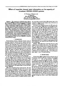
3.5 Numerical Results and Discussions Throughout this section the propagation loss is modeled as β = (d/d0 )−m [67], where d is the distance between the transmitter and receiver, d0 is the reference distance, and m is the path loss exponent. The following results are based on d0 = 1km and m = 2.7, which corresponds to urban area cellular networks. The relays’ distances from the source and destination, d[sr] = d[rd] = 1km unless otherwise specified. The channel gains from source antennas to relays and relays to destination antennas are modeled as i.i.d complex Gaussian random variables with CN (0, 1). Walsh-Hadamard codes of length L = 8 combined with BPSK modulation are used during the training interval. During the data transmission interval the VBLAST proposed in [106] is employed, where QPSK modulation is used with a frame length of 128, resulting in an overall estimation overhead of 6%. A minimum of 1000 Monte-Carlo trials are used. Finally, SNR is defined as 1/σv2 and 1/σw2 for both source-relay and relay-destination links, respectively. Fig. 3.2 presents the mean-square error (MSE) of the ML and LS channel estimators for R = {4, 6} relays, M = N = {2, 4}, and L = 16, where the MSE plot for
39
0
MSE for Channel Estimation
10
LS, M=N=2, R=4 ML, M=N=2, R=4 Gao et al. M=N=2, R=4 LS, M=N=4, R=6 Gao et al. M=N=4, R=6
−1
10
MSE for ML and LS estimators for R=4 relays
−2
10
0
2
4
6
8
10
12
14
16
18
20
SNR [dB]
Figure 3.2: Comparison of the proposed channel estimators for AF relaying networks vs. the estimator in [23].
the MLE for R = 6 relays is omitted, since it is similar to the case of LS. Moreover, the performance of the proposed estimators are compared against the LS estimator in [23], where time division multiple access (TDMA) is used at the source antennas to extend the results in [23] to the case of MIMO cooperative networks. The training sequence length is set to L = 8, which is chosen to ensure a fair comparison, since the estimator in [23] requires twice the number of time slots compared to the ML and LS estimators proposed in this chapter. Fig. 3.2 illustrates that both the MLE and LS algorithms proposed in this chapter outperform the estimator in [23] by an average margin of 2dB. Note that the LS method requires O(L) multiplications per S-D antenna pair while the MLE requires at least O(L3 ) multiplications
40
due to the L × L matrix inversions. 6
5
b/s/Hz
4
3 AF, R=3 AF, R=6 AF, R=8 APSF, R=3 APSF, R=6 APSF, R=8
2
1 AF capacity for R=3, 6, and 8. 0 0
5
10
15
20
25
30
SNR [dB]
Figure 3.3: Capacity of the 2-hop cooperative network for both AF and APSF with R = {3, 6, 8} relays and M = N = 2.
Fig. 3.3 illustrates the capacity of the two-hop cooperative network for AF and APSF. It is shown that unlike AF in the case of APSF, addition of relays to the network results in significant capacity gains. This considerable performance gap is caused by the fact that the signals from multiple relays are coherently combined at the destination due to the phase shift applied by APSF. Note that a comparison between APSF and the schemes in [15, 45, 48, 86, 94, 111] is not made, since the algorithms proposed in [15, 45, 48, 86, 94, 111] require the estimation of sourcerelay and relay-destination links channel gains separately, which adds significantly more training overhead and hardware complexity at the relays.
41
0
10
ABER for AF with R=4 and 6 relays
−1
10
−2
ABER
10
−3
10
−4
10
−5
10
−6
10
0
AF, R=2, Perfect CSI AF, R=4, Perfect CSI AF, R=6, Perfect CSI APSF, R=2, Perfect CSI APSF, R=4, Perfect CSI APSF, R=6, Perfect CSI AF, R=4, Estimated CSI APSF, R=4, Estimated CSI APSF, R=6,Estimated CSI 5
10
15
20
25
30
SNR [dB]
Figure 3.4: BER performance of AF and APSF for the case perfect and estimated CSI. R = {2, 4, 6} relays, M = N = 2, training length, L = 8 and frame length=128.
Fig. 3.4 shows the average-bit-error-rate (ABER) for AF and APSF relaying cooperative networks in the presence of perfect and estimated CSI for R = {2, 4, 6} relays. The iterative Golden Section (GS) search algorithm is stopped after 10 iterations. Fig. 3.4 illustrates that in the case of AF relaying, increasing the number of relays from 4 to 6 does not result in any noticeable cooperation gain, similar to the results in Fig. 3.3. The results in Fig. 3.4 illustrate that in cases of both perfect and estimated CSI, APSF results in performance gains of 5dB and 8dB compared to AF when the cooperative network is equipped with 4 and 6 relays, respectively. Note
42
that for clarity, the plot for AF relaying with R = 6 and estimated CSI is omitted, since it is the same as for the case of R = 4. AF APSF, Iterations=1 APSF, Iterations=5 APSF, Iterations=10
−1
10
−2
ABER
10
−3
10
APSF for 5 and 10 iterations
−4
10
−5
10
0
5
10
15
20
25
30
SNR [dB]
Figure 3.5: ABER of APSF when the number of iteration for the Golden Section search algorithm is set to 1, 5, and 10 vs. SNR for R = {4} relays.
Fig. 3.5 presents the ABER plots for an APSF relaying cooperative network with R = 4 relays when the GS search algorithm’s number of iterations is fixed at 1, 5, and 10. Fig. 3.5 illustrates that the proposed GS algorithm converges very quickly (in 5 iterations in this scenario), where the majority of the performance gain is achieved with very few iterations, e.g., after 1 and 5 iteration APSF relaying delivers a 5dB and 8dB performance gain, respectively, compared to AF relaying in the mid SNR region. The plots for the case of estimated CSI are not presented, since APSF also converges very quickly in the case of imperfect CSI. Fig. 3.6 investigates the performance of APSF in the case of quantized phase 43
AF APSF, 1 bit APSF, 2 bits APSF, 3 bits APSF Unlimited bits
−1
10
−2
ABER
10
−3
10
−4
10
ABER for 3 and unlimited bits −5
10
0
5
10
15
20
25
SNR [dB]
Figure 3.6: Comparison of ABER of APSF and AF for uniformly quantized phase values vs. SNR for K = {4} relays.
values. A uniform quantizer is used at the destination limiting the amount of feedback to the relays. The results in Fig. 3.6 illustrate that the phase shifts at the relays can be represented using a 2 or 3 bit quantizer without any significant performance loss due to the effect of quantization. This result can be compared against the investigations outlined in [26] for CSI quantization. Fig. 3.7 represents a comparison between APSF and AF when relays are at different geographical locations. Positions 1, 2 , and 3 refer to relays that are 1, 2, and 3 kms away from source, respectively, and d[sr] + d[rd] = 4kms. Fig. 3.7 illustrates that the performance gains promised by APSF are still attainable, even if the relays
44
0
10
−1
10
−2
ABER
10
−3
10
−4
10
−5
10
0
AF(1 1 3 3) AF(1 1 1 1) AF(3 3 3 3) AF(2 2 2 2) APSF(2 2 2 2) APSF(1 1 1 1) APSF(3 3 3 3) APSF(1 1 3 3) 5
10
15
20
25
30
SNR [dB]
Figure 3.7: ABER of AF and APSF when the relays are distributed at different locations within the network. Positions 1, 2 , and 3 refer to relays that are 1, 2, and 3 kms away from S, respectively (see Fig. 3.1, R = 4, M = N = 2).
45
are distributed throughout the network. Note that since the results presented in Fig. 3.7 are scenario dependent, more general quantitative conclusions regarding relays’ locations and ABER performance cannot be made.
3.6 Conclusions In this chapter, new training methods and algorithms for estimation of channel gains in AF relaying MIMO cooperative networks are presented. A new training method that allows for simultaneous estimation of the overall channel gains from source to destination in 2-hop multi-relay cooperative networks are derived. Numerical results show that the proposed LS and ML channel estimators outperform the existing algorithms. Next, a new distributed beamforming algorithm for the optimization of multirelay MIMO cooperative networks is outlined that is shown to result in significant performance gain in realistic settings. The performance gains promised by APSF are achieved with minimal added feedback, since the proposed algorithm only requires the set of quantized phases to be fed back to the relays and does not add to the channel estimation overhead already required by AF relaying networks. Moreover, the computational overhead at the destination is minimal due to the fact that the iterative Golden Section search algorithm converges quickly. Finally, even though employing APSF entails additional hardware and requires the application of phase shifts at the relays, the required hardware can be implemented using simple digital signal processing algorithms.
46
Chapter 4 Effects of Timing Jitter and Frequency Offset on System Performance
4.1 Introduction
TIMING jitter and frequency offset represent important communications systems parameters that often require estimation and compensation. As a result, the estimation accuracy of these parameters greatly affects the performance of communications systems. This chapter seeks to determine quantitative bounds on the performance of communications systems in the presence of imperfect timing and frequency offset estimation. The Cramer-Rao lower bound (CRLB) is the lower bound on the variance of an unbiased estimator of unknown parameters [44]. Here, unknown parameters refer to the absence of any assumed statistical distributions. For applications to communication signals, evaluation of the CRLB is further complicated by unknown
47
nuisance parameters, e.g., the problem of determining the CRLB for frequency offset estimation for a signal received in white Gaussian noise in the presence of unknown phase offset. To overcome this, a more easily evaluated modified CramerRao lower bound (MCRLB) is proposed in [1], though it is a looser bound [113]. Classically, inter-symbol interference (ISI) is determined as a function of a given timing offset. Performance may be depicted graphically in the form of the wellknown eye diagram as illustrated in Fig. 2.2. Characterizing the effect of timing error normally assumes that a deterministic slowly varying component can be tracked and compensated for with well-understood signal processing algorithms such as the Gardner detector (GD) [25, 55]. The unknown, uncompensated timing offsets give rise to a source of random fluctuation in the received signal-to-noise ratio (SNR). Quantifying the effect of timing error is difficult. One approach is to simply calculate the received SNR for every possible timing offset and then average the result, yielding an average-bit-error-rate (ABER) [3,4]. This approach, while straightforward in principle, is dependent upon receiver signal processing algorithm, e.g., sampling rate, matched filter, decision device, etc. Also problematic is the dependence of the above approach on an assumed probability distribution of the timing offset, which is completely unknown in practice. The alternative approach taken in this thesis is to determine the inherent effects of design decisions such as pulse shape, signal bandwidth, carrier separation, etc. using a non-random, unknown model of timing offset on system performance, independent of receiver algorithm, by generalizing and extending techniques that determine variance lower bounds.
48
The effect of frequency offset on the performance of orthogonal frequency division multiplexing (OFDM) systems has been extensively researched in the literature and is summarized in [70]. Fractional frequency offsets with respect to the subcarrier spacing results in inter carrier interference (ICI) and SNR loss at the receiver which has been quantitatively analyzed in [70] and [41]. However, the variance or even bounding the variance of the SNR loss due to ICI has not been addressed to date. As outlined in [1] and [113], the CRLB for frequency offset estimation is complicated due to unknown phase offset and channel fading. A lower bound on the variance of SNR due to ICI is determined by analyzing the properties of the MCRLB under functional transformation. Next, the outage probability for OFDM systems due to frequency offset is analyzed. In [2], the outage probability versus signal-to-interference ratio (SIR) is determined for an OFDM system based on Monte-Carlo simulations. In this chapter, using the derived lower bound on the variance of SNR with respect to frequency offset, a closed-form expression for the outage probability as a function of frequency offset for OFDM systems is numerically calculated. The idea of functional transformation for the CRLB appears in [44]. In this chapter, we first generalize the results in [44] to functional transformations for the MCRLB, and then apply them to determine the lower bound on the variance of signal pulse estimation due to timing offset for different types of pulses, including raised cosine (RC) [73], root-raised cosine (RRC) [33], and flipped exponential (FEX) [4] [3]. The new approach, however, is not restricted to these three pulses but can be generalized to other pulse designs. The functional transformation for the MCRLB is also used to determine a lower bound for the variance of SNR due to frequency offset. The derived lower bound on SNR uncertainly is applied to assess
49
outage probability. Finally, the relationships between the MCRLB and CRLB under different synchronization scenarios are determined, as well as necessary conditions for the CRLB and the MCRLB to be equivalent. This chapter is organized as follows: Section 4.2 derives the MCRLB for discretetime signals in additive white Gaussian noise. Section 4.3 derives a general expression for functional transformation of the MCRLB. Section 4.4 applies the functional transformation of the MCRLB to derive a lower bound on the estimation signal pulse and SNR as a function of timing offset and frequency offset, respectively. Finally, Section 4.5 analyzes the applicability of the MCRLB as a lower bound for the estimation of synchronization parameters by comparing it against the CRLB.
4.2 Modified CRLB The modified Cramer-Rao lower bound (MCRLB) for continuous-time signals was proposed in [1]. In this section we derive the MCRLB for discrete-time signals received in white Gaussian noise. Recall that the Cramer-Rao lower bound (CRLB) can be expressed as CRLB(λ) , −
[ Er
1 ∂ 2 ln p(r|λ) ∂λ2
]=
[( Er
1 ∂ ln p(r|λ) ∂λ
)2 ] ,
(4.1)
where E{·} represents the expectation with respect to p(r, λ), and ln(·) represents the natural logarithm function. For (4.1) to hold, the PDF p(r, λ) must satisfy the regularity condition [44, 79] (note that strictly speaking there are four regularity conditions that (4.2) arises from [79]) [ Er
] ∂ ln p(r|λ) = 0. ∂λ
50
(4.2)
Assuming n = 0, 1, · · · , L − 1
r[n] = s[n; λ] + w[n]
(4.3)
is observed in white gaussian noise (WGN), the conditional probability of r given the parameter of interest λ, termed the likelihood function, is represented as { } N −1 1 1 ∑ 2 p(r|λ) = exp |r[n] − s[n; λ]| . (4.4) (2πσ 2 )N/2 2σ 2 n=0 Differentiating p(r|λ) once results in N −1 ∂ ln p(r|λ) 1 ∑ ∂s[n; λ] = 2 |r[n] − s[n; λ]| . ∂λ σ n=0 ∂λ
A second differentiation results in [ ( )2 ] N −1 ∂ 2 ln p(r|λ) ∂s[n; λ] 1 ∑ ∂ 2 s[n; λ] = 2 |r[n] − s[n; λ]| − . ∂λ2 σ n=0 ∂λ2 ∂λ
(4.5)
(4.6)
Taking the expectation with respect to r results in ( Er
∂ 2 ln p(r|λ) ∂λ2
) =−
N −1 1 ∑ ∂ 2 s[n; λ] . σ 2 n=0 ∂λ2
(4.7)
Applying (4.1), 2 ˆ ≥∑ σ 2 var(λ) . N −1 ∂ s[n;λ] n=0
(4.8)
∂λ2
Now suppose instead that the PDF p(r|λ) is also dependent on a set of extraneous parameters u, expressed as p(r|λ, u), then to determine the CRLB(λ), p(r|λ, u) needs to be first averaged over the unwanted parameters via ∫
−∞
p(r|λ) =
p(r|λ, u)p(u)du. ∞
(4.9)
Determining the CRLB is further complicated in this case, since to evaluate (4.9), assumptions regarding the distributions of the nuisances parameters, u, need to 51
be made. In addition, due to the fact that (4.9) is a multi-dimensional integration, evaluating it, unfortunately is not easy for most distributions. Thus, to avoid carrying out (4.9), the following modified CRLB, where from here on is denoted as the MCRLB, is given by [(
MCRLB(λ) = Er,u
1 ∂ ln p(r|λ,u) ∂λ
)2 ] ,
(4.10)
is proposed in [1]. The MCRLB is derived based on [1] [( Er,u
ˆ −λ λ(r)
)2 ]
[
[(
= Eu Er|u ≥ Eu
Er|u [(
Eu Er|u [(
= Er,u
)2 ]]
[(
[
≥
ˆ −λ λ(r) 1
∂ ln p(r|λ,u) ∂λ
1 ∂ ln p(r|λ,u) ∂λ
1 ∂ ln p(r|λ,u) ∂λ
] )2
)2 ]]
)2 ] ,
(4.11)
where the first inequality in (4.11) follows from the properties of the CRLB and the second inequality is based on Jenson’s inequality and convexity of the
1 x
function
for x > 0. According to (4.11), it can be deduced that the MCRLB is a lower bound on the CRLB and is a looser lower bound on the variance of an unbiased estimator. In the case of synchronization parameter estimation, Section 4.5 determines the set of conditions that need to be met for the CRLB and MCRLB to coincide. Using (4.7) and (4.10), we express the discrete MCRLB for a signal transmitted in white Gaussian noise as [ Er,u
[N −1 ] ] ∑ ∂ 2 s[n; λ, u] ∂ 2 ln p(r|λ, u) 1 = − 2 Eu . 2 ∂λ2 σ ∂λ n=0 52
(4.12)
Therefore, an alternative to (4.8) is given by ˆ ≥ var(λ)
Eu
[∑
σ2 N −1 ∂ 2 s[n;λ,u] n=0 ∂λ2
].
(4.13)
Note that (4.7) and (4.12) differ by the expectation term Eu (·). The MCRLB can ˆ denoted as f (λ), ˆ as described also be extended to arbitrary smooth functions of λ, in Section 4.3.
4.3
MCRLB under functional transformation
In this section we derive the MCRLB for a parameter β = f (λ) whose probability distribution function (PDF) is parameterized by λ. We consider all unbiased estimators, i.e. those for which ˆ = β. f (λ) = Er [β]
(4.14)
After differentiating both sides ∂f (λ) = ∂λ
∫
∂p(r|λ) βˆ ∂r ∂λ ∫ ∫ ∂p(r|λ, u) = p(u)∂r∂u βˆ ∂λ ] [∫ ∂p(r|λ, u) = Eu βˆ ∂r ∂λ [∫ ] ∂ ln p(r|λ, u) ˆ = Eu β p(r|λ, u)∂r . ∂λ
(4.15)
In addition, due to the regularity condition (4.2), we have [∫ Eu
] ∫ ∂ ln p(r|λ, u) ∂ ln p(r|λ) β p(r|λ, u)∂r = β p(r|λ)∂r ∂λ ∂λ [ ] ∂ ln p(r|λ) = βEr ∂λ = 0. 53
(4.16)
Using (4.16), (4.15) can be rewritten as ∂f (λ) = Eu ∂λ
[∫
] ∂ ln p(r|λ, u) ˆ (β − β) p(r|λ, u)∂r . ∂λ
(4.17)
Squaring both sides (
∂f (λ) ∂λ
)2
[∫ ≤ Eu
]2 ∂ ln p(r|λ, u) ˆ (β − β) p(r|λ, u)∂r , ∂λ
(4.18)
where the inequality in (4.18) follows from Jensen’s inequality and the convexity of φ(x) = x2 . The Cauchy-Schwarz inequality can be applied to (4.18) (
∂f (λ) ∂λ
)2
[∫
]2 ∂ ln p(r|λ, u) ≤ Eu (βˆ − β) p(r|λ, u)∂r ∂λ [ [ ]]2 ∂ ln p(r|λ, u) = Eu Er|u (βˆ − β) ∂λ [ [( )2 ]] [ ] ∂ ln p(r|λ, u) ≤ Eu Er|u (βˆ − β)2 Er|u ∂λ ] [( )2 ∂ ln p(r|λ, u) ˆ u,r . = var(β)E ∂λ
(4.19)
From (4.19), the variance of βˆ can be lower bounded as ( )2 [(
ˆ = MCRLB(β) Er,u
∂f (λ) ∂λ
∂ ln p(r|λ,u) ∂λ
)2 ] ,
(4.20)
which is the required generalization of the MCRLB of λ given in (4.10).
4.4 Applications of the Functional Transformation of the MCRLB In this section the functional transformation of the MCRLB, derived in Section 4.3, is applied to derive a quantitative relationship between the lower bound on estimation of synchronization parameters and performance of communications systems. 54
4.4.1 Effect of Timing offset on the RC, RRC, and FEX Pulses In a baseband pulse amplitude modulation (PAM) system the received waveform is first passed through a matched filter and is then sampled at the symbol rate, where the optimum sampling times correspond to the peaks of the signal pulses [66]. Therefore, the accuracy by which the signal pulse can be estimated has a direct impact on the performance of a communications system. In this subsection, we apply the MCRLB to derive the lower bound on the variance of estimating the raised-cosine (RC), root-raised cosine (RRC) [33], and flipped exponential (FEX) [3, 4] signal pulses in the presence of timing offset.
4.4.1.1
The Raised-Cosine (RC) Pulse
The RC signal pulse, gRC , as a function of the timing offset, τ , is given by gRC (τ ) =
sin(πτ /T ) cos(απτ /T ) , πτ /T 1 − 4α2 τ 2 /T 2
(4.21)
where T is the symbol duration and α is the roll-off factor. The roll-off factor, α, is a measure of the excess bandwidth of the filter, i.e. the bandwidth occupied beyond the Nyquist bandwidth of
1 2T
[33]. If the excess bandwidth is denoted by ∆f , then α = 2T ∆f.
Using (4.21) and (4.20), the lower bound on the variance of estimating the RC signal pulse as a function of timing offset, gRC (τ ), can be determined as (
∂gRC (τ ) ∂τ
)2
1 × MCRLB (gRC (τ )) = 2 , Es T2 8π LξRC N 0
(4.22)
where L denotes the length of the observation interval, in symbols, Es /N0 is the SNR, and the normalized mean-square bandwidth of the RC pulse, ξRC , is defined 55
as ξRC ,
∫∞ 2 f |GRC (f )|2 df 2 −∞ ∫ T ∞ |GRC (f )|2 df −∞
Note that GRC (f ) in (4.23) is given by 1, [ ( πT [ 1 GRC (f ) = 1 + cos |f | − 2 α 0,
(4.23)
.
|f | ≤ 1−α 2T
])]
,
1−α 2T
1−α 2T
< |f | ≤
1+α 2T
(4.24)
otherwise.
After simple algebraic manipulation, ξRC is calculated to be ξRC = In addition, in (4.22),
∂gRC (τ ) ∂τ
1 12
−
α 16
+
α2 4
3
+ 5α − 16 α 1− 4
2α2 π2
+
α3 8π 2
.
(4.25)
can be evaluated as
cos( απτ )( πτ cos( πτ ) − sin( πτ )) ∂gRC (τ ) T T T T = 2 1−4α2 τ 2 πτ ∂τ ( T ) ) (T 8α2 τ πα απτ απτ ) sin( ) cos( ) sin( πτ 2 T T − T 1−4α2 τ 2 T . − πτT 1−4α2 τ 2 2 ) ( 2 2 T T T
(4.26)
Fig. 4.1 depicts the MCRLB of estimating the RC signal pulse, MCRLB(gRC (τ )), versus timing offset for different values of roll-off factor, α. Note that in Fig. 4.1, MCRLB(gRC (τ )) more slowly increases as the timing offset increases for larger rolloff factor values. This indicates that in the presence of timing offset, the RC signal pulse and its peak can be more accurately estimated for larger roll-off factor values. This reduces the effect of ISI due to timing offset, which is also shown qualitatively using eye diagrams in [66].
4.4.1.2 Root-Raised Cosine (RRC) Pulse In the case of RRC pulse, (4.20) can be reused to derive the lower bound on the variance of estimating the RRC signal pulse in the presence of timing offset, MCRLB− 56
0.4 SNR=10, α=0, L=10 SNR=10, α=.5, L=10 SNR=10, α=1, L=10
0.35
MCRLB(gRC(τ))
0.3
0.25
0.2
0.15
0.1
0.05
0 −0.5
−0.4
−0.3
−0.2
−0.1
0
0.1
0.2
0.3
0.4
0.5
Normalized Timing Offset
Figure 4.1: MCRLB(gRC (τ )) for the RC pulse, with L = 10, SNR=10dB, and α = {0, .5, 1}.
(gRRC (τ )). Note that the RRC signal pulse, gRRC , as a function of the timing offset, τ , is given by
( sin gRRC (τ ) =
(1−α)πτ T
π Tt
) (
+
( ) cos (1+α)πτ T , ( 4ατ )2 )
4ατ T
1−
(4.27)
T
where similar to (4.21), the roll-off factor, α, is a measure of the excess bandwidth. Using (4.27),
∂gRRC (τ ) ∂τ
∂gRRC (τ ) = ∂τ +
can be expressed as ( (1+α)πτ (1+α)π sin( ) 4B T − − πT T
128α3 πT 3
(
( cos
(1+α)πτ T
(
(1 −
)
τ 1−
T 4ατ
(1−α)πτ
T sin( T 4ατ 2
( 4ατ )2
+ sin ) ( 4ατ )2 2 T
57
(T
)
)
(1−α)πτ T
+
(1−α)πτ T
(1−α)π cos( 4ατ
)
)
)) .
(4.28)
Finally, to determine the MCRLB(gRRC (τ )), the normalized mean-square bandwidth, ξRRC , also needs to be determined. Note that GRRC (f ) =
√
GRC (f ),
(4.29)
where GRC (f ) is defined in (4.24). Using (4.29) and GRRC (f ) instead of GRC (f ) in (4.23), the normalized mean-squared bandwidth for the RRC pulse, after simple algebraic manipulations is calculated as ξRRC =
(1 + 3α2 ) 2α2 − 2 . 12 π
(4.30)
Fig. 4.2 plots the lower bound on the variance of RRC signal pulse estimation in the presence of timing offset, MCRLB(gRRC (τ )), for different roll-off factor values. Note that similar to the results in Fig. 4.1, as the roll-off factor, α, increases, MCRLB(gRRC (τ )) more slowly increases with the timing offset. Therefore, it can be concluded that RRC signal pulse timing can be more accurately estimated for larger roll-off factor values, which also agrees with observations in [66].
4.4.1.3 Flipped Exponential (FEX) pulse According to eye diagram plots and average-bit-error-rate (ABER) simulations in [3, 4], compared to the RC pulse, the flipped exponential (FEX) pulse has been found to improve system performance in the presence of timing offset. Here, we derive the lower bound on the estimation variance of FEX pulse, MCRLB(gFEX (τ )), and quantitatively compare the results with those of the RC and RRC pulses. The FEX signal pulse, gFEX , as a function of the timing offset, τ , is given by gF EX (τ ) = sinc(τ /T )
4βπτ sin(πατ /T ) + 2β 2 cos(πατ /T ) − β 2 , (2πτ )2 + β 2
58
(4.31)
1.8 SNR=10, α=1, L0=10 SNR=10, α=.5, L =10
1.6
0
SNR=10, α=0, L0=10
1.2
MCRLB(g
RRC
(τ))
1.4
1 0.8 0.6 0.4 0.2 0 −0.5
−0.4
−0.3
−0.2
−0.1
0
0.1
0.2
0.3
0.4
0.5
Normalized Timing Offset
Figure 4.2: MCRLB(gRRC (τ )) for the RRC pulse, with L = 10, SNR=10dB, and α = {0, .5, 1}.
where β =
2T ln 2 . α
∂gFEX (τ ) = ∂τ − + −
Using (4.31),
cos( πτ ) T τ
(
∂gFEX (τ ) ∂τ
can be derived as
4βπτ sin( πτTα ) + 2β 2 cos( πτTα ) (4π 2 τ 2 + β 2 )
1/2 sin( πτ ) T (4βπτ πτ 2 B 1/2 sin( πτ ) T (4βπ πτ B 4π sin( πτ ) T (4βπτ B
)
sin( πτTα ) + 2β 2 cos( πτTα ) − β 2 ) (4π 2 τ 2 + β 2 )
sin( πτTα ) + 8βπ 2 τ Bα cos( πτTα ) − 4β 2 πBα sin( πτTα )) (4π 2 τ 2 + β 2 ) sin( πτTα ) + 2β 2 cos( πτTα ) − β 2 ) . (4π 2 τ 2 + β 2 )2
(4.32)
Next, (4.23) and the frequency domain representation of the FEX pulse, GF EX (f ),
59
given by 1, ( ( )) exp β 1−α − |f | , 2T GF EX (f ) = ( ( )) 1+α 1 − exp β |f | − , 2T 0,
|f | ≤
1−α 2T
1−α 2T
< |f | ≤
1 2T
1 2T
< |f | ≤
1+α 2T
(4.33)
otherwise,
are used to determine the normalized mean-square bandwidth of the FEX pulse, ξF EX , which after simple algebraic manipulations is calculated as ξF EX =
1 24
+ .0225α + .34169α2 + .20137α3 . α .5 − 8 ln(2)
(4.34)
Fig. 4.3 depicts the lower bound on the variance of FEX signal pulse estimation, MCRLB(gFEX (τ )), for different roll-off factor values. Comparing the results in Figs. 4.1 and 4.3, it is clear that for the same value of timing offset and rolloff, α, the MCRLB(gFEX (τ )) is smaller than that of MCRLB(gRC (τ )). This indicates that in the presence of timing offset, the FEX’s signal pulse can be more accurately estimated compared to that of the RC pulse. Therefore, it can be concluded that the application of the FEX pulse in a communications system reduces the effect of ISI due to timing offset and improves system performance. This quantitative results agrees with qualitative eye diagrams and ABER results presented in [3, 4]. Note that a more fair comparison between the lower bound on the variance of RC, RRC, and FEX signal pulse estimation based on the normalized square bandwidth is performed in Section 4.4.1.4.
4.4.1.4 Performance Comparison of the RC, RRC, and FEX Pulses In this section we compare the MCRLB(g(τ )) for the RC, RRC, and FEX pulses. Fig. 4.4 A. illustrates that for the same roll-off factor values, α, the FEX pulse results in 60
0.35
SNR=10, α=0, L0=10 SNR=10, α=.5, L =10 0
0.3
SNR=10, α=1, L =10 0
MCRLB(gFEX(τ))
0.25
0.2
0.15
0.1
0.05
0 −0.5
−0.4
−0.3
−0.2
−0.1
0
0.1
0.2
0.3
0.4
0.5
Normalized Timing Offset
Figure 4.3: MCRLB(gFEX (τ )) for the FEX pulse, with L = 10, SNR=10dB, and α = {0, .5, 1}.
a lower variance for the estimation of the signal pulse when compared to the RC and RRC pulses. From the MCRLB plots in Fig. 4.4 A. it can be concluded that the lower bound for the estimation of the FEX signal pulse in the presence of timing offset is smaller than that of the RC and RRC pulses, which indicates that the FEX signal pulse can be estimated with higher accuracy in the presence of timing offset. This result, which also supports the qualitative results observed in [3, 4, 33], show that the application of the FEX pulse reduces ISI due to timing offset and improves system performance. While Fig. 4.4 A. performs the comparison in a manner consistent with that
61
A. 0.7
α=.35, RC α=.35, RRC α=.35, FEX
0.6
0.6
0.5
0.5
0.4
0.4
MCRLB
MCRLB
B. 0.7
0.3
0.3
0.2
0.2
0.1
0.1
0 −0.5 −0.4 −0.3 −0.2 −0.1
0
0.1 0.2 0.3 0.4 0.5
ξ=.09, RC ξ=.09, RRC ξ=.09, FEX
0 −0.5−0.4−0.3−0.2−0.1
0
0.1 0.2 0.3 0.4 0.5
Normalized Timing Offset
Normalized Timing Offset
Figure 4.4: A. MCRLB(gRC (τ )), MCRLB(gRRC (τ )), and MCRLB(gFEX (τ )) with L = 10, SNR=10dB, and for the same roll-off factor, α = .35. B. MCRLB(gRC (τ )), MCRLB(gRRC (τ )), and MCRLB(gFEX (τ )) with L = 10, SNR=10dB, and the same normalized mean-square bandwidth ξ=.09.
presented in [4] and [3], we now present a more appropriate comparison based on the normalized mean square bandwidth as defined in (4.23). Fig. 4.4 B. compares the RC, RRC, and FEX pulses for ξRC = ξRRC = ξF EX = .09. As shown in Fig. 4.4 B. the FEX pulse still outperforms both the RC and RRC pulses but not by as large of a margin as the somewhat misleading results indicate in Fig. 4.4 A.
4.4.2 Effect of Frequency Offset on OFDM Systems The effect of inter carrier interference (ICI) causing frequency offset on the performance of orthogonal frequency division multiplexing (OFDM) systems is briefly summarized in Section 2.4. In this section the effect of CFO estimation uncertainty 62
on SNR uncertainty is determined. Let us denote the SNR of an OFDM system with perfect and imperfect frequency offset estimation by SNR[ideal] and SNR[real] , respectively. The relationship between SNR[ideal] , SNR[real] , and frequency offset, ν, in an OFDM system containing Ns subcarriers is shown to be [70] γdB (ν) =
SNR[ideal] SNR[real]
( = 10 log
) { } 1 2 1 + SNR[1 − fNs (ν) ] , fNs (ν)2
(4.35)
where γdB (ν) is a measure of SNR loss due to frequency offset and fNs (x) =
sin(πx) . Ns sin(πx/Ns )
(4.36)
Using (4.20), the lower bound on the estimation of γdB (ν) in the presence of frequency offset, ν, can be determined using ( MCRLB(γdB (ν)) =
∂γdB (ν) ∂ν
)2
Es 2 L(L − 1)2 N T /3 0
,
(4.37)
where L represents the length of the pilot signal in symbols and Es /N0 is the SNR. Note that to derive (4.37), the MCRLB of estimation of ν in [1] and the functional transformation of the MCRLB in (4.20) are used. In (4.37),
∂γdB (ν) ∂ν
can be derived as
∂γdB (ν) 10 sin2 (πν) ( ( )) = sin2 (πν) 2 ∂ν 2 ln(10)Ns sin (πν/Ns ) 1 + Es /N0 1 − N 2 sin2 (πν/Ns ) s [ ( ( )) −2Ns2 π cos(πν) sin2 (πν/Ns ) sin2 (πν) × 1 + Es /N0 1 − 2 2 sin3 (πν) Ns sin (πν/Ns ) )) ( ( 2Ns π cos(πν/Ns ) sin(πν/Ns ) sin2 (πν) + 1 + Es /N0 1 − 2 Ns sin(πν/Ns )2 sin2 (πν) )] ( Ns2 sin2 (πν/Ns )Es /N0 −2π sin(πν) cos(πν) 2π cos(πν/Ns ) sin2 (πν) , + + sin2 (πν) Ns2 sin2 (πν/Ns ) Ns3 sin3 (πν/Ns ) (4.38)
63
Using the relationships in (4.35) and (4.38) the probability of outage for an OFDM system as a function of frequency offset can be determined. The probability of outage here is defined as Poutage = p(SNR[real] < SNRT ),
(4.39)
where SNRT represents the target threshold SNR for acceptable system performance. Approximating the outage distribution as Gaussian, (4.39) can be lower bounded as ( Poutage = Q where σdB (ν) =
γdB (ν) − SNRT σdB (ν)
) ,
(4.40)
√ MCRLBν (SNR) is determined using (4.37), and tail probability ∫ Q(z) = z
∞
1 2 √ e−y /2 dy. 2π
(4.41)
Fig. 4.5 A. plots SNR[real] vs. frequency offset for different SNR[ideal] values using (4.35). Fig. 4.5 B. plots MCRLB(γdB (ν)) vs. frequency offset, and Fig. 4.5 C. depicts the lower bound on probably of outage using (4.40) for different SNR[ideal] values when SNRT is set to 0dB. In the calculations of outage probability, the MCRLB is used to determine the lower bound on SNR variance. The length of the observation interval L = 5 is motivated by the short training sequence used in IEEE 802.11a [89]. Even though in [70] and references therein, the mean SNR loss due to ICI causing frequency offset is extensively analyzed, the effect of frequency offset on the variance of SNR has been mainly ignored. The approach outlined above allows for a quantitative method of determining the variance of lower bound on the variance of SNR due to frequency offset in OFDM systems. 64
A.
B.
10 SNR
10
C.
0
6 =5
ideal
SNRideal=7.5 5
σ2SNR[real] > MCRLB(SNR)dB
mean of SNR
[real]
(dB)
8 7 6 5 4
SNR
=10
−1
ideal
10
Lower bound on Poutage
9
4
3
2
−2
10
−3
10
−4
3
10 1
2 1 −2 10
−1
10
−5
0 −2 10
−1
10
Normalized Frequency Offset ν Normalized Frequency Offset ν
10
−1
10
Normalized Frequency Offset ν
Figure 4.5: In the above figures we consider an OFDM system with Ns =512 and L=5. A. SNR vs. normalized frequency offset based on (4.35). B. MCRLB(SNR) vs. normalized frequency offset using (4.37) and (4.38). C. Poutage vs. normalized frequency offset with SNRT =0dB according to (4.40).
Note that when compared to the CRLB, the MCRLB is a looser lower bound on the variance of an unbiased estimator. Therefore, to justify the application of the MCRLB as lower bound for the estimation of synchronization parameters, we show, in the following section, that in some important practical scenarios, the CRLB and MCRLB coincide.
65
4.5 MCRLB vs. CRLB for Synchronization Parameter Estimation Although the MCRLB and CRLB have been used in the literature, the difference between the two bounds for estimating synchronization parameters has not been carefully addressed. In this section, it is demonstrated that the MCRLB coincides or is close to the CRLB for synchronization parameter estimation in many practical situations and that the simplicity associated with the MCRLB justifies its use in circumstances where calculation of the CRLB is difficult. This section also shows that timing and frequency offset estimation in communications systems can be decoupled from one another. This result is applied in Chapters 5 and 6 to simplify the analyses for synchronization parameter estimation in multi-relay cooperative communications systems and separately address multiple timing and frequency offsets estimation. For joint vector parameter estimation, λ = [λ1 , λ2 , · · · , λp ], the CRLB for the estimation of the ith component λi is given by [44] [ ] CRLB(λi ) = FIM−1 (λ) i,i ,
(4.42)
where FIM(λ) is the p×p Fisher’s information matrix (FIM). Note that the elements of FIM(λ), fλi ,λj , for i, j = 1, 2, · · · , p, are given by ] [ 2 ∂ ln p(r, λ) . fλi ,λj = −E ∂λi ∂λj
(4.43)
To derive the MCRLB for the estimation of λi , the remaining parameters λj , for j = 1, 2, · · · , j ̸= i, · · · , p, are assumed to be nuisance parameters. Based on definition (4.11), the MCRLB for the estimation of λi is expressed as [30] MCRLB(λi ) =
1 , Eu [fλi ,λi ] 66
for
i = 1, 2, · · · , p
(4.44)
where in this case the vector of nuisance parameters, u = [λ1 , λ2 , · · · , λj̸=i , · · · , λp ]. By comparing (4.42) and (4.44), it can be deduced that if the off-diagonal elements of the FIM are zero, i.e., [fλi ,λj ] = 0 for i ̸= j, then the estimation of λi , for i = 1, 2, · · · , p, can be decoupled and the CRLB and MCRLB are equivalent. Let us determine the CRLB and MCRLB for the joint estimation of synchronization parameters for a signal received in zero-mean white Gaussian noise (WGN) using (4.42) and (4.44), respectively. The continuous-time received signal, r(t), for a passband communication system can be expressed as r(t) =
L−1 ∑
sn g(t − nT − τ T )ej(νkT +θ) + v(t),
(4.45)
n=0
where L is the length of the sequence in symbols, sn are data symbols belonging to some M -ary constellation, g(t) is an even-symmetric real-valued transmitted pulse, τ represents the timing offset, ν is the frequency offset, θ is the phase offset, and v(t) is the zero-mean additive white Gaussian noise (AWGN) with variance N0 . Here, the joint estimation of λ = [τ, ν, θ] is considered. The FIM for the joint estimation of timing, frequency, and phase offset can be written as
fτ,τ fτ,ν fτ,θ FIM(λ) = fν,τ fν,ν fν,θ fθ,τ fθ,ν fθ,θ
.
(4.46)
Since the focus is on determining the difference between the CRLB and MCRLB, we only discuss the off-diagonal elements of the FIM(λ) matrix in (4.46). In (4.46), fτ,ν , fτ,ν , and fτ,ν are given by [67] {∫ fτ,ν = fν,τ = −LT ℑ
∞
−∞
} ∗
(t + τ )g (t)g(t)dt × SNR,
67
(4.47)
{∫ fτ,θ = fθ,τ = −LT ℑ
∞
−∞
} ∗
g (t)g(t)dt × SNR,
(4.48)
and [
∫
fν,θ = fθ,ν = L τ T +
∞
−∞
] t|g(t)| dt × SNR, 2
(4.49)
where ℑ denotes the imaginary part. Given that g(t) is real-valued pulse in most communication systems, the terms in (4.47) and (4.48) vanish. Therefore, FIM(λ) can be rewritten as
0 fτ,τ 0 FIM(λ) = 0 fν,ν fν,θ 0 fθ,ν fθ,θ
.
(4.50)
Based on (4.50), it can be concluded that the estimation of timing offset can be decoupled from frequency offset and phase offset estimation. This result corroborates existing contributions presented in [25], which show that in the case of a Gardner detector, timing offset estimation can be performed accurately in the presence of frequency offset. In addition, we can conclude that the MCRLB and CRLB for the estimation of timing offset, τ , are equivalent. This shows that the MCRLB is a valid and tight lower bound on the variance of timing offset estimators. Even though the CRLB and MCRLB for the estimation of τ are the same under the above assumptions, the two bounds are very different under the consideration of Rayleigh fading channels [49], with the MCRLB being considerably easier to determine. On the other hand, the CRLB can only be determined under specific scenarios. For details on the determination of the CRLB and MCRLB for fading channels, see [49].
68
For frequency offset and phase offset estimation based on the fact that offdiagonal elements fν,θ and fθ,ν in (4.49) are non-zero, we can conclude that compared to the CRLB, the MCRLB for frequency offset estimation is a looser lower bound. However, for real-valued even-symmetric signals, g(t), the integral in (4.49) is equal to zero and as the timing offset, τ , goes to zero the terms fν,θ and fθ,ν vanish. Therefore, we can conclude that under the assumption of perfect timing synchronization, the MCRLB and CRLB for phase and frequency offset estimation are equivalent.
4.6 Conclusions In this chapter, the functional transformation for the modified CRLB is derived and is applied to determine lower bounds on the estimation of signal pulse amplitude and SNR as a function of timing and frequency offset, respectively. Unlike MonteCarlo based comparisons, e.g., eye-diagrams and ABER plots that are dependent on simulation parameters, the derived closed-form expressions can be applied to quantitatively determine the effect of different system parameters on the performance of communications systems. Next, the relationship between the MCRLB and CRLB under different synchronization scenarios is determined, where it is demonstrated that the MCRLB is a tight lower bound for most practical scenarios. In addition our analysis demonstrates that timing and frequency offset estimation in communications systems can be decoupled and investigated as two separate problems. As a result, in Chapters 5 and 6 we separately address the topics of multiple timing and frequency offsets estimation in distributed cooperative networks.
69
Chapter 5 Timing Offset Estimation in Distributed Cooperative Networks
5.1 Introduction
EVEN though many cooperative strategies have been proposed that provide full spatial diversity in the presence of multiple timing offsets, they result in reduced transmission rates and/or also require timing offsets to be accurately estimated for effective detection and equalization (see, e.g., [53, 90, 115] and references therein). In this chapter we seek to address timing synchronization using a training sequence in distributed amplify-and-froward (AF) and decode-and-forward (DF) cooperative networks. Due to the distributed nature of the network and simultaneous transmissions from separate nodes with different oscillators, cooperative networks require the estimation of multiple timing offsets to combat the resulting inter-symbol interference (ISI) and signal-to-noise ratio (SNR) loss [66, 67]. Moreover, even though multi-input-single-output (MISO) systems are a critical component of cooperative communication networks, the timing offset estimation algorithms available in the 70
literature for MISO systems, e.g., [57,72,82,107] are not applicable in the case of cooperative communication systems, due to the existence of multiple timing offsets. In [38, 63, 74] the effect of timing synchronization errors on the performance of cooperative relay networks is analyzed, where it is demonstrated that timing offsets much smaller than the symbol interval can result in considerably higher pair-wise error probabilities. In [37] it is shown that in the case of multi-relay DF cooperative networks, as the number of relays increases, timing synchronization errors have an adverse effect on the signal-to-interference-noise ratio (SINR) and outage probability of cooperative networks. Thus, achieving timing synchronization via accurate multiple timing offset estimation algorithms is key to future deployments of cooperative networks. Several algorithms are proposed for accurate timing offset estimation in the case of point-to-point single-input-single-output (SISO) systems [24, 25, 55, 67, 71]. In [67], the maximum-likelihood estimator (MLE) for timing offset estimation in the case of SISO systems is presented. In [25] Gardner proposes an estimator that can accurately determine the timing offset between the transmitter and receiver at considerably lower computational complexity compared to the MLE in [67]. Papers [55] and [24] further enhance the performance of Gardner’s detector. Timing offset estimation in the case of point-to-point multiple-input-multiple-output (MIMO) systems is addressed in [57, 72, 82, 107], where it is shown that achieving timing synchronization in MIMO systems comes at higher overhead and complexity. In [54] the topic of timing synchronization in DF cooperative networks is considered, where the emphasis is on timing offset compensation. Even though an
71
MLE-based multiple timing offset estimator for DF cooperative networks is presented, the proposed estimator has a very high computational complexity, since it entails solving an R-dimensional maximization problem, where R is the number of relay nodes. Moreover, to achieve timing synchronization the proposed MLE requires each relay’s timing offset to not exceed one symbol timing duration, which is not justifiable in the case of cooperative networks consisting of multiple distributed relays with different oscillators. Finally, [54] does not analyze or investigate the effect of the training sequence and network topology on timing estimation performance. To the best of the author’s knowledge, timing offset estimation in AF cooperative networks has not been addressed to date. In [60] frequency offset estimation in distributed DF and AF relaying multirelay cooperative networks is addressed. However, the Cramer-Rao lower bounds (CRLBs) and estimators proposed in [60] are not applicable to the case of timing offset estimation due to the considerably different signal model. Moreover, unlike the results in [60], as outlined in this thesis, to achieve timing synchronization in distributed cooperative networks, timing offsets need to be estimated at both the relays and destination in both cases of DF and AF relaying cooperative networks. Finally, accurate timing offset estimation entails specific training sequence design that is different from the case of frequency offset estimation. The CRLB [44] is used as a quantitative benchmark for the performance of timing offset estimators [39,54,55,57,72] and [93]. Moreover, the CRLB can be applied to determine the effect of network protocol, topology, choice of training sequence, and number of relays on timing offset estimation accuracy in cooperative systems. The CRLB of timing offset estimation for point-to-point SISO systems is derived in [39], where it is demonstrated that the choice of training sequence significantly
72
impacts estimation accuracy. In [93] the CRLB for the estimation of timing offset using an array of antennas is derived and it is shown that the CRLB can be reached at mid-to-high SNR. In [57], results in [93] are extended to the CRLB for timing offset estimation in Gaussian and Rayleigh flat-fading channels for MIMO systems. In [54] the CRLB for timing offset estimation in DF cooperative networks is derived, but the analysis is limited to the case of Gaussian channels and closed-form expressions are not provided. This chapter first derives the CRLBs for timing offset estimation for DF and AF multi-node cooperative systems for Rician fading and Gaussian channels. In the case of AF, a new low complexity baseband processing structure is proposed that enables accurate joint multiple timing offsets estimation at the destination. The CRLBs are used to design more effective training sequences and to determine the effect of number of relays and relay locations on timing offset estimation in distributed DF and AF cooperative networks. Next, an iterative multiple timing offset estimator is proposed that transforms the R-dimensional maximization problem into R single parameter estimation problems that can then be solved using the 1-dimensional MLE, Gardner’s detector, or Mueller and Muller estimator [71]. As a result, the proposed multiple timing offset estimator significantly reduces the computational complexity and overhead required for achieving timing synchronization in multi-relay cooperative networks. Furthermore, the proposed estimator is capable of estimating timing offsets much larger than one symbol duration and simulation results show that its performance approaches or reaches the CRLB at low, mid, and high SNR. Note that in [54], it has been shown that when combined with re-synchronization filters, timing offset estimators that reach the CRLB significantly improve the ABER of multi-relay distributed cooperative networks.
73
This chapter is organized as follows: in Section 5.2, the system model for the cooperative system is presented, Section 5.3 derives the CRLBs for DF and AF relaying. In Section 5.4 the effect of training sequence on the CRLB is analyzed and the proposed training sequence design for multi-relay cooperative networks is outlined. Section 5.5 overviews the MLE for timing offset estimation, outlines the iterative multiple timing offset estimator, and analyzes the complexity of the proposed algorithm. Section 5.6 presents numerical results that investigate the effect of number of relays, training sequence, and network topology on timing synchronization in cooperative networks and compares the performance of the proposed estimator against the CRLB.
5.2 System Model A half-duplex cooperative network consisting of a source and destination pair and a cluster of R relay nodes is considered, where the relays are assumed to be distributed throughout the network as shown in Fig. 5.1 A. As illustrated in Fig. 5.1 B. transmission is divided into two intervals: i) training interval and ii) data transmission interval. In this chapter, multiple timing offset estimation using a training sequence is analyzed, where during the training interval the timing offsets and channel gains corresponding to the R relay nodes are estimated. These estimates can be applied in the data transmission interval to mitigate inter-symbol interference (ISI) and improve system performance. Throughout this chapter the following set of assumptions and system design parameters are considered: 1. In Phase I, the source broadcasts its training sequence to the relays. In Phase II 74
to efficiently estimate the timing offsets, the relays transmit R distinct training sequences simultaneously to the destination (see Fig. 5.1). 2. Timing offsets are modeled as unknown non-random parameters. 3. The effect of carrier frequency offset (CFO) on the received training signal is not considered since as discussed in [28] and Chapter 4, timing offset estimation can be decoupled from CFO estimation. Refer to Chapter 6 or [60] for a detailed analysis of the topic of frequency synchronization in distributed multi-relay cooperative networks. 4. Colored zero-mean additive Gaussian noise (AGN) is considered at the relays and destination. 5. Without loss of generality, it is assumed that unit-amplitude phase-shift keying (PSK) training sequences are transmitted. Note that Assumptions 2 and 3 are in line with previous timing offset estimation analyses performed for point-to-point systems in [39, 54, 57, 72, 82, 107] and are also intuitively justifiable, since the main sources of timing offset are oscillator mismatch and channel delay [67]. Both of these effects are assumed to not significantly change throughout the short training sequence. Assumption 4 ensures that the results in this chapter are applicable to a wide range of scenarios, e.g., when timing offset estimation is performed after matched filtering, the resulting noise is not white [39].
75
Figure 5.1: A. The system model for the cooperative network. B. Scheduling diagram for training and data transmission intervals.
5.2.1 Training Signal Model at the Relays The sampled baseband received training signal, prior to the matched filter, rk (iTs ), at the kth relay, 1 ≤ k ≤ R is given by rk (iTs ) =
√
p[s] h
L−1 ∑ k
[sr]
t[s] (n)g(iTs − nT − τk T ) + vk (iTs ),
(5.1)
n=0
where: • L and T denote the length of the training sequence and the symbol duration, respectively, • T = Nt Ts , where Ts is the sampling time and Nt is the number of samples per symbol,
76
• t[s] (n) is the known nth training symbol broadcast from the source to the relays, [sr]
• τk
is the normalized timing offset from the source to the kth relay,
• hk represents the unknown channel gain from the source to the kth relay that is assumed to not change over the interval n = 1, 2, · · · , L, • p[s] is the transmitted power from the source, and • vk (n) is the AGN at the kth relay with mean zero and variance σv2k , which is denoted by CN (0, σv2k ). Eq. (5.1) can be represented in matrix and vector form as rk =
√
[sr]
p[s] hk Gk t[s] + vk ,
(5.2)
where: • rk , [rk (0), rk (1), · · · , rk (Nt L − 1)]T , • t[s] , [t[s] (0), t[s] (1), · · · , t[s] (L − 1)]T , • vk , [vk (0), vk (1), · · · , vk (Nt L − 1)]T , and ] [ [sr] [sr] • Gk is an Nt L × L matrix, where Gk
m,l
[sr]
, g(mTs − lT − τk T ).
Note that the subsequent sections assume that after estimation and compensa[ ] [sr] [sr] tion of the timing offsets τ [sr] , τ1 , · · · , τR at the relays, the residual offsets propagate to the destination where they are estimated and mitigated.
77
5.2.2 Training Signal Model at the Destination for DF Relaying Cooperative Networks The decode-and-forward (DF) protocol requires the signals at the relays to be decoded and timing offsets, τ [sr] to be estimated and equalized at the relays. Therefore, t[s] received in Phase I is used for timing offset estimation similar to that of a point-to-point single-input-single-output (SISO) system as shown in Fig. 5.2. Moreover, to ensure successful cooperation in Phase II, the estimated timing offsets, τ [sr] , are applied to align the relays’ transmissions in time with respect to the source. Note that the timing corrector in Fig. 5.2 is similar to a voltage-controllable delay line, which produces synchronized samples [66]. Unlike Phase I, in Phase II or the cooperation phase, the superposition of training signals received from the relays must be used to jointly estimate the timing offsets [ ] [rd] [rd] from the relays to the destination, τ [rd] , τ1 , · · · , τR .
Figure 5.2: Block diagram of the baseband receiver at the kth relay for DF networks.
The sampled baseband received training signal model, y , [y(0), y(1), · · · , y(Nt
78
L − 1)]T , for a DF cooperative network consisting of R relay nodes is given by y=
R (√ ∑
) [r] [rd] [r] pk fk Gk tk
(5.3)
+ w,
k=1
where: [rd]
• Gk
[ ] [rd] is an Nt L × L matrix, where Gk
[rd]
m,l
[rd]
, g(mTs − lT − τk T ) and τk
is the normalized timing offset from the kth relay to the destination, [r]
[r]
[r]
• tk , [tk (0), · · · , tk (L − 1)]T is the known transmitted training sequence specific to the kth relay, • fk represents the unknown channel gain from the kth relay to the destina[r]
tion that is assumed to not change over the interval n = 1, · · · , L, pk is the transmitted power from the kth relay, and • w , [w(0), w(1), · · · , w(Nt L − 1)]T is the zero mean AGN at the destination with w(n) distributed as CN (0, σw2 ) and the covariance matrix of w denoted by Σw .
5.2.3 Training Signal Model at the Destination for AF Relaying Cooperative Networks To enable synchronous transmission and successful cooperation in Phase II, similar to DF, in AF networks the relays need to estimate timing offsets from the source to the relays, τ [sr] , where the training sequence transmitted from the source in Phase I can be used similar to that of a point-to-point SISO system. Furthermore, to ensure accurate timing offset estimation at the destination, the kth relay’s transmitted training signal needs to be distinct for 1 ≤ k ≤ R. Hence, to achieve timing
79
synchronization throughout an AF relaying cooperative network, we propose the baseband processing structure in Fig. 5.3 at the relays. Note that the block diagram in Fig. 5.3 suggests a considerably simpler implementation compared to that of DF networks in Fig. 5.2, since the received signal at the relays does not need to be matched filtered, decoded, and encoded before retransmission.
Figure 5.3: Block diagram of the proposed baseband processing at the kth relay for timing estimation and compensation in AF networks.
Using the AF relay processing indicated in the block diagram in Fig. 5.3 and the fact that the received signal vector at the kth relay, rk , is amplified and forwarded without being decoded, the sampled baseband representation of the received training signal model at the destination in Phase II is given by y(iTs ) =
L−1 R ∑ ∑
[sd]
[r]
|k=1 n=0 +
R ∑
[rd]
pk ζk fk hk t[s] (n)tk (i)g(iTs − nT − τk T ) {z √
ζk
}
desired signal [r]
pk fk v˜k (iTs ) + w(iTs ),
|
{z
k=1
(5.4)
}
overall noise
where: [r]
[r]
• v˜k (iTs ) , vk (iTs )tk (i) and tk (i) is the ith symbol of the kth relay’s training sequence, 80
√ [sd] • ζk , 1/ p[s] |hk |2 + σv2k satisfies the kth relay’s power constraint, and pk , √ [r] pk p[s] . Eq. (5.4) can be represented in matrix and vector form as √ R R ( ) ∑ ∑ [sd] [rd] [s] [r] [r] y= ζk pk fk hk Gk t ⊙ tk + ζk pk fk v ˜k + w, [r]
[
k=1 [r]
[r]
where tk , tk (0), , · · · , tk (Nt L − 1)
]T
(5.5)
k=1
as shown in Fig. 5.3, ⊙ denotes the Schur
(element-wise) product, and v ˜k , [˜ vk (0), v˜k (1), · · · , v˜k (Nt L − 1)].
5.2.4 Multiple Timing Offset Estimation in Cooperative Networks In Phase I of the training interval, timing offset estimation at the relays is similar to that of point-to-point SISO systems, which has been extensively investigated in the literature (e.g., see, [39] and [25]). However, in Phase II, since the asynchronous training signals from R relay nodes are received simultaneously at the destination, the timing offsets, τ [rd] in (5.3) and (5.5), need to be jointly estimated. Despite the simpler overall baseband processing structure, timing offset estimation in the case of AF relaying is actually very complicated due to the more complex training signal model at the destination as noted in (5.5). To date the MLE proposed in [81] and [54] are the only methods of determining the timing offsets in the case of distributed cooperative networks. Even though joint MLE can in principle accurately estimate timing offsets, its computational complexity is extremely high and is not amenable to practical implementation. Therefore, in this chapter we propose a multiple timing offset estimation algorithm that seeks to reduce the overhead associated with timing synchronization in distributed cooperative networks. Since the CRLB is used as a benchmark to assess the performance of the proposed estimators, we first derive the CRLB. 81
5.3 Cramer-Rao Lower Bound In this section, the CRLB for timing offset estimation for DF and AF multi-relay cooperative networks is derived. Note that since the channel gains are assumed to be unknown, for more a complete analysis the CRLBs need to be derived for the joint estimation of both timing offsets and channel gains. However, the CRLB expressions for the joint estimation of these 3R parameters (R real and imaginary part of channel gains and R timing offsets) are too complex and provide little insight on the effect of training sequence, network protocol, and topology on timing offset estimation. As a result, in this section the CRLB expressions for the joint estimation of the R timing offsets are derived. Numerical results in Section 5.6 show that the CRLBs derived in this section are tight and are reached by the proposed estimators in Section 5.5. Note that the numerical results in Section 5.5 assume unknown and estimated channels.
5.3.1 Decode-and-Forward Cooperative Networks The general case of Rician fading channels is considered, where the channel gain from the kth relay to the destination, fk , is modeled as a Gaussian random variable with mean and variance µfk and σf2k , respectively. Note that Rayleigh fading represents the special case where the mean line-of-sight path has zero power. [ ] [rd] [rd] [rd] According to (5.3), for DF networks the set of timing offsets, τ = τ1 , · · · , τR needs to be jointly estimated at the destination. For notational clarity, (·)[DF] is used instead of (·)[rd] below. Derivation of the CRLB for the joint estimation of τ [DF] : For notational convenience the following variables are defined
82
• Df , diag
(√
[r] p1 µf1 ,
) √ √ [r] [r] p2 µf2 , · · · , pR µfR is an R × R matrix,
[ ] [DF] is an Nt L × R matrix, δ [DF] , ∂ξ[DF] /∂τk = • ∆[DF] , δ [DF] , δ [DF] , · · · , δ [DF] 1 2 R k k ∂G[DF] [r] k [DF] tk , ∂τ k
[r]
• ξ [DF] , G[DF] k k tk , and ( [DF] )H ( [DF] )H • Γ[DF] , δ [DF] ξk + ξ [DF] δk is an Nt L × Nt L matrix. k k k Under the stated assumptions, y is distributed as y ∼ CN (µy , Σy ), where µy = E[y] =
R √ ∑
[r]
pk µfk ξ[DF] , k
and
(5.6a)
k=1
Σy = E[(y − µy )(y − µy ) ] = H
R ∑
( [DF] )H [r] pk σf2k ξ[DF] ξk + Σw . k
(5.6b)
k=1
To determine the CRLB, the R × R Fisher’s Information Matrix (FIM) needs to be determined. In the case of parameter estimation in a complex Gaussian observation sequence, the entries of FIM are given by [44] [ ] [ ] ∂µH ∂µ y y −1 −1 Σy −1 Σy FIM(λ)k,m = 2Re Σ + Tr Σy Σ , ∂λk y ∂λm λk y λm
(5.7)
[ ] [DF] [DF] [DF] where λ = τ1 , τ2 , · · · , τR , √ [r] = pk µfk δ [DF] , and k
(5.8)
( ( [DF] )H ( [DF] )H ) [r] [r] [DF] = pk σf2k δ [DF] ξ + ξ δk = pk σf2k Γ[DF] . k k k k
(5.9)
∂µy [DF]
∂τk ∂Σy [DF]
∂τk
Note that δ [DF] is dependent on the choice of the transmitted pulse, g(t), in (5.1). k Using (5.7), (5.8), and (5.9) the entries of the FIM are determined as [ ] FIM(τ [DF] ) k,m =2Re
{√ } ( [DF] )H −1 [DF] [r] [r] ∗ pk pk µfk µfm δ k Σy δ m 83
[ ] [r] −1 [DF] −1 [DF] 2 2 + Tr pk p[r] σ σ Σ Γ Σ Γ . m fk fm y y m k
(5.10)
Let FIMDF = FIM(τ [DF] ). Then the CRLB for the estimation of τ [DF] is given by the diagonal elements of the inverse of FIMDF , which are calculated as { } CRLBR (τ [DF] ) = diag FIM−1 DF {( { )−1 } ( [DF] )H −1 [DF] } H [DF] = diag 2Re Df ∆ Σ y ∆ Df + Υ ,
(5.11)
where the elements of the R × R matrix Υ[DF] are given by ] [ [ [DF] ] [r] [r] 2 2 −1 [DF] −1 [DF] σ Σ Γ Σ Γ . Υ , Tr p p σ y m k m fk fm y k k,m
(5.12)
Note that in the case of additive white Gaussian noise (AWGN) and slow fading channels, σf2k = 0, for 1 ≤ k ≤ R, the covariance matrix of the observation vector, y, Σy = σw2 I. Therefore, Υ[DF] in (5.12) vanishes to zero and the CRLB simplifies to { 2 ( { } ( [DF] )H [DF] })−1 σw H [DF] CRLBG (τ ) = diag Re Df ∆ ∆ Df . (5.13) 2 Based on (5.11) and (5.13) the following remarks are in order: (
[r]
[r]
1. When the same training sequence is transmitted from all the relays t1 = t2 ) [r] = · · · = tR and timing offsets from the relays to the destination are approx( ) imately the same τ1[DF] ≃ τ2[DF] ≃ · · · ≃ τR[DF] , the matrix FIMDF becomes singular, pointing to the fact that an unbiased estimator does not exist (see, e.g., [91]) and the CRLBs in (5.11) and (5.13) approach infinity. Therefore, the training sequences transmitted from each relay needs to be linearly independent to ensure accurate timing offset estimation. This is investigated further in Section 5.4. 2. Using (5.13) it can be shown that the application of orthogonal training sequences minimizes the CRLB and improves estimation performance. More details are provided in Sections 5.4 and 5.6. 84
3. In the case of R = 1 and AWGN, the CRLBs in (5.11) and (5.13) simplify to CRLBR (τ
[DF]
{( } ) σw2 ( [DF] H −1 [DF] 2 Σy δ ) = [r] |µf | Re δ 2p [ ( )2 ])−1 [DF] −1 [DF] + Tr p[r] σf4 Σ−1 Γ Σ Γ , and y y
σ2 CRLBG (τ [DF] ) = − [r]w 2 2p |f | respectively, where g¨(t) =
(
L ∑
g¨(nT )
n=−L
∂ 2 g(t) ∂t2
L ∑
(
)∗ t[r] (i) t[r] (i − n)
(5.14)
)−1 ,
(5.15)
i=−L
and for notational convenience, t[r] (x) , 0
for x < 0 and x ≥ L. Eq. (5.15) is the closed-form expression for the CRLB for the estimation of τ [DF] and is similar to the CRLB in [39]. 4. Note that an expression similar to (5.15) may represent the CRLB for the es[sr]
timation of τk
at the kth relay, where the parameters corresponding to the
source to relay link are used instead.
5.3.2 Amplify-and-Forward Cooperative Networks For AF relaying cooperative networks under the consideration of Rician or Rayleigh frequency-flat fading channels, there does not exist an explicit CRLB expression for the estimation of timing offsets, τ [rd] , due to the presence of the term fk hk in (5.5) and since the product of two Gaussian random variables is not Gaussian and its probability distribution function (PDF) is very difficult to calculate, [20]. Thus, in this chapter the CRLB is derived for the case of quasi-static fading channels, where hk and fk are assumed to not change over the length of training sequence. Zeromean AGN is considered, where v ˜k and w are distributed according to CN (0, Σv˜k ) and CN (0, Σw ), respectively. Moreover, v ˜k , v ˜m , and w are assumed to be mutually independent for k ̸= m and ∀k, respectively. 85
[ ] [rd] [rd] According to (5.5), the set of R timing offsets, τ [rd] = τ1 , · · · τR needs to be jointly estimated at the destination. For notational clarity, (·)[AF] is used instead of (·)[rd] . Derivation of the CRLB for the joint estimation of τ [AF] : For notational convenience the following variables are defined [sd]
• Dα , diag(α1 , · · · , αR ) is an R × R matrix, αk , ζk pk fk hk , βk , ζk
√
[r]
pk fk , [AF]
[AF] • ∆[AF] , [δ [AF] , δ [AF] , · · · , δ [AF] , ∂ξ [AF] 2 R ] is an Nt L × R matrix, δ k k /∂τk ( )1 ∂G[AF] [r] [s] k ⊙ tk , and [AF] t
=
∂τk
) ( [r] [s] • ξ [AF] , G[AF] ⊙ tk . k k t Based on the above definitions, (5.5) can be rewritten as y=
R ∑
αk ξ [AF] k
+
k=1
R ∑
βk v ˜k + w.
(5.16)
k=1
According to (5.16), y, is distributed as y ∼ CN (µy , Σy ),
(5.17)
where µy = Σy =
R ∑ k=1 R ∑
αk ξ [AF] k
(5.18a)
|βk |2 Σv˜k + Σw .
(5.18b)
k=1
To determine the CRLB, the R×R FIM according to (5.7) needs to be determined ] [ [AF] [AF] [AF] where λ = τ1 , τ2 , · · · , τR , ∂µy = αk δ [AF] (5.19) k , and [AF] ∂τk ∂Σy [AF]
∂τk
86
= 0.
(5.20)
Using (5.7), (5.19), and (5.20) the entries of the FIM are determined as { [ ] ( )H −1 [AF] } FIM(τ [AF] ) k,m = 2Re αk∗ αm δ [AF] Σy δ m . k
(5.21)
Let FIMAF = FIM(τ [AF] ). Then the CRLB for the estimation of τ [AF] is given by the diagonal elements of the inverse of FIMAF , which are calculated as {( } { { } ( [AF] )H −1 [AF] })−1 −1 H [AF] CRLBR (τ ) = diag FIMAF = diag 2Re Dα ∆ Σy ∆ Dα . (5.22) In the case of AWGN, where v ˜k and w are distributed according to CN (0, σv˜2k I) for k = 1 · · · R and CN (0, σw2 I), respectively, the covariance matrix of y simplifies to Σy =
( R ∑(
)
)
|βk |2 σv˜2k + σw2
(5.23)
I.
k=1
Subsequently, the CRLB in (5.22) can be rewritten as { ∑R ( } ) 2 2 2 ( { }) −1 ( ) |β | σ + σ k v˜k w k=1 [AF] H CRLBG (τ [AF] ) = diag 2Re DH ∆[AF] Dα . α ∆ 2 (5.24) Based on (5.22) the following remarks are in order: [r]
1. For R = 1 the training sequence at the relay can be set to tk = [1, 1, · · · , 1], and the CRLB in (5.24) can be expressed in closed-form as ( L )−1 L 2 2 2 ∑ ∑ ( ) |β| σ + σ ∗ v˜ w CRLBG (τ [AF] ) = g¨(nT ) t[s] (i) t[s] (i − n) , (5.25) 2 2|α| n=−L i=−L where for notational convenience, t[s] (x) , 0 for x < 0 and x ≥ L. 2. Based on (5.24), similar to DF relaying, to accurately estimate the timing offset for each relay node (nonsingular FIMAF ), the transmitted training signals from each relay need to be distinct, ξ [AF] ̸= ξ[AF] ̸= · · · ̸= ξ [AF] 1 2 R . 87
5.4 Training Sequence Design Throughout this section it is assumed that BPSK signaling is used for the transmission of the training sequences.
5.4.1 Training Sequence Design for DF Relaying Networks We first show that orthogonal training sequences such that ( )2 [r] ∑L ( )H k=i t (n) i n=1 [r] [r] tk , k = 1···R ti = 0 k ̸= i
(5.26)
result in a reduced CRLB for the estimation of the timing offsets from the relays to the destination, τ [DF] . In the case of DF relaying cooperative networks, under the assumption of real transmitted pulses, g(t), the CRLB in (5.13) can be rewritten as CRLBG (τ
[DF]
) = diag
{
FIM−1 DF
}
{ = diag
σw2 2
( )} (( )−1 ( ) ) −1 [DF] H [DF] H −1 Df ∆ ∆ Df . (5.27)
Note that for most communications systems, g(t), is real. Moreover, (5.27) follows from the facts that the diagonal elements of the FIM are real for real transmitted pulses, g(t) and Df is a diagonal matrix. ( )H Theorem 5.1: The CRLBG in (5.27) is minimized, when the matrix Ω , ∆[DF] ∆[DF] is diagonal. Proof: According to (5.27), minimizing the CRLB for the estimation of τ [DF] is equivalent to minimizing the trace of the matrix CRLBG . Moreover, based on results in [44], for an M × M positive definite matrix X the following holds, M ] ∑ [ Tr X−1 ≥ j=1
88
1 , [X]jj
(5.28)
with equality if X is diagonal. Let us assume that the optimum Ω that minimizes [ ] Tr CRLBG (τ [DF] ) is not diagonal. Then, based on (5.27), we can conclude that FIMDF is also not diagonal. Using (5.28) we obtain that M [ ] [ ] ∑ Tr CRLBG (τ [DF] ) = Tr (FIMDF )−1 ≥ j=1
1 . [FIMDF ]jj
(5.29)
g DF = diag {FIMDF } that results in a According to (5.29), there exists a matrix FIM [ ] lower Tr CRLBG (τ [DF] ) . This leads to a contradiction. Hence, the optimum Ω must be diagonal. (
Note that Ω , ∆
) [DF] H
[ ∆
[DF]
[DF]
and ∆
=
∂G[DF] [r] 1 [DF] t1 , · · · ∂τ 1
,
∂G[DF] [r] R [DF] tR ∂τ
]T . Since
R
the matrices G[DF] , · · · , G[DF] are unknown as they are a function of the unknown 1 R timing offsets, τ [DF] , the known training sequences must be designed in a such a fashion to lower the off-diagonal elements of Ω and minimize the CRLB. Numerical analysis in Section 5.6 show that transmission of orthogonal training sequences, when combined with the set of all possible timing offsets, lowers the CRLB. In practice point-to-point communication systems often use sign-alternating preambles or training sequences to improve timing offset estimation [25, 67]. Although the complexity of the CRLB expressions for multi-relay cooperative communications systems in (5.11) and (5.22) makes it very difficult to analytically show that training sequences that alternate in sign from one symbol to another such that [r]
ti (n) = (−1)n
(5.30)
result in a lower CRLB, numerical analysis observed in Section 5.6 indicate that under the assumption of Nyquist transmitted pulses, g(t), the alternating one-zero sequence results in the lowest possible CRLB in the case of multiple timing offset estimation. This is also empirically justifiable since Gardner’s detector and the
89
timing offset estimators proposed in [25] and Section 5.5 also perform better if the continuous signal pulse changes sign from one symbol to another. The Walsh-Hadamard an orthogonal family of codes. The Walsh-Hadamard matrix is a square matrix with dimensions of 2k , for k = 1, 2, 3, · · · , and entries of +1 or −1. The Walsh-Hadamard matrices are given by the recursive relationship [42, 68]
(
)
(
)
W 2 ( k−1 ) ( ) W 2 W 2k = . ( k−1 ) ( k−1 ) = W (2) ⊗ W 2 W 2 −W 2 k−1
k−1
(5.31)
Even though satisfying both conditions (5.26) and (5.30) is not possible, wellperforming training sequences can be designed based on Walsh-Hadamard codes using the following steps: 1. Select Walsh-Hadamard code sequences of length Lt , sk = [sk (0), sk (1), · · · , sk (Lt − 1)] with emphasis on selecting the code sequences that alternate in sign the most. [r]
2. The orthogonal training sequence, tk , for k = 1, 2, · · · .R is designed such that [r]
tk = [sk (0), sk (1), · · · , sk (Lt − 1), · · · , sk (0), sk (1), · · · , sk (Lt − 1)]T , | {z }
(5.32)
L
where by repeating shorter codewords of length Lt , training sequences of length L can be constructed without a performance penalty. Therefore, log2 R < Lt ≤ L. For example let us consider R = 4, L = 64, Nt = 2, and Lt = 8. Then L=64
•
[r] t1
L=64
z }| { z }| { [r] T T = [1, −1, 1, −1, 1, −1, 1, −1, · · · ] , t2 = [1, −1, −1, 1, −1, 1, 1, −1, · · · ] , | {z } | {z } s1
s2
90
[r]
[r]
• t3 = [1, 1, −1, −1, 1, 1, −1, −1, · · · ]T , and t4 = [1, −1, −1, 1, 1, −1, −1, 1, · · · ]T . | {z } {z } | s3
s4
5.4.2 Training Sequence Design for AF Relaying Networks Similar steps to that of Subsection 5.4.1 can be used to show that orthogonal training sequences also result in a lower CRLB and improve the estimation performance in the case of AF relaying cooperative networks. Therefore, Walsh-Hadamard code sequences can be used to design good training sequences for AF relaying networks. For example let us consider R = 2, L = 64, Nt = 2, and Lt = 8. Then L=64
• t[s]
z }| { = [−1, 1, −1, 1, −1, 1, −1, 1, · · · ]T , L×N =128
[r]
• t1
L×N =128
t t z }| { }| { z [r] = [1, −1, 1, −1, 1, −1, 1, −1, · · · ]T , and t2 = [1, −1, −1, 1, −1, 1, 1, −1, · · · ]T . | | {z } {z }
s1
s2
Note that as shown in (5.5) in the case of AF relaying, the choice of the training sequence transmitted from the source, t[s] affects timing offset estimation performance at the destination.
5.5 Proposed Timing Offset Estimator In this section, a brief overview of the MLE for multiple timing offset estimation is provided. More details can be found in [54, 93]. Next, the proposed multiple timing offset estimators, iterative-MLE (I-MLE) and iterative-Gardner detector (I-GD) are outlined. Throughout this section the following assumptions are made: • The number of relays, R, and training sequences are assumed to be known at the destination,
91
• AWGN noise is assumed at all terminals, • the noise at each relay and destination are assumed to be mutually mutually independent, • similar to the results in [39, 54, 57, 72, 82, 107], quasi-static fading channels are considered, where channel gains are assumed to be constant over the length of the training sequence, and • the channel gains are assumed to be unknown at the receiver, since in practical communication systems, timing offset estimation is performed priori to channel estimation [67]. For readability purposes, the case of DF cooperative networks is discussed first and to simplify notation τ [DF] is represented by τ .
5.5.1 MLE for Multiple Timing Offset Estimation In order to determine the MLE for timing offset estimation we first need to determine the joint log-likelihood function (LLF) of timing offsets and channel gains. Assuming that the received signal at the destination, y, is Gaussian distributed, the LLF is proportional to y = Ξ[DF] (τ )η + w, where: • η,
[√
[r] p1 f1 ,
]T √ √ [r] [r] p2 f2 , · · · , pR fR ,
[ ] • Ξ[DF] (τ ) , ξ [DF] , ξ [DF] , · · · , ξ[DF] , and ξ [DF] is defined in Section 5.3.1. 1 2 R k Note that Ξ[DF] (τ ) and ξ[DF] , for k = 1, · · · , R, are both functions of τ . k
92
(5.33)
Using the fact that the vector of received training signals, y, is a Gaussian random variable, the LLF ρ(τ , η) is given up to an additive constant by
2 ρ(τ , η) = y − Ξ[DF] η .
(5.34)
It is a well known fact that for a given τ , the minimizer of (5.34) is given by ˆ= η
((
Ξ[DF]
)H
Ξ[DF]
)−1 (
Ξ[DF]
)H
(5.35)
y.
Inserting (5.35) into (5.34), the timing offset estimates can be obtained as τˆ [DF] = arg max yH Ξ[DF] τ
((
Ξ[DF]
)H
Ξ[DF]
)−1 (
Ξ[DF]
)H
y,
(5.36)
where in Matlab notation the set of possible timing offsets, τ = {τ1 · · · τR } can be represented as τk ∈ {−ϵk : ∆τk : ϵk } for 1 ≤ k ≤ R,
(5.37)
with [−ϵk , ϵk ) and ∆τk denoting the range and step size for the timing offset corresponding to the kth relay, respectively. Based on (5.36) the following remarks are in order: 1. As the timing offset values become close to one another (τ1 ≃ τ2 ≃ · · · ≃ τR ) and the transmitted training sequences become more highly correlated, the )−1 (( )H going to infinity in MLE does not exist due to the term Ξ[DF] Ξ[DF] (5.36). This outcome is consistent with the CRLB results in Section 5.3. 2. The maximization in (5.36) is very complex, since it is R-dimensional and requires carrying out large size matrix multiplications and inversion. This will be discussed in more detail in Subsection 5.5.5. Moreover, even though the application of the iterative alternating projection method outlined in [117] can reduce the complexity of MLE, it still requires evaluating (5.36) at every iteration. 93
3. To accurately estimate each relay’s timing offset and reach the CRLB the step size for the maximization in (5.36) needs to be small. For example to obtain useful accuracy, it is required that ∆τk ≤ 10−4 , for 1 ≤ k ≤ R, resulting in a large set of possible timing offsets, further increasing the overall complexity of the MLE. 4. When new relays are added to the network or when the nodes within the network require re-synchronization, the complex R-dimensional maximization in (5.36) needs to be performed again.
5.5.2 I-MLE for DF Networks To address the above shortcomings, we propose an iterative MLE (I-MLE). While estimating the mth relay’s timing offset, I-MLE uses initial estimates of the timing offsets and knowledge of the training sequences to eliminate the signal corresponding to the remaining relays. Based on this approach the training signal model in (5.3) can be rewritten as ) (√ √ R ∑ [r] [r] [DF] [r] [DF] [r] y = pm fm Gm tm + pk fk Gk tk + |{z} w . | {z } k=1,k̸=m noise desired term | {z }
(5.38)
interference
Note that by using the alternating projection method [117] and large initial step sizes, e.g., ∆τk = 5 × 10⁻² for 1 ≤ k ≤ R, the maximization in (5.36) can be used to calculate rough initial estimates of the timing offsets, (ˆ τ )[1] , where due to the significantly smaller set of possible values the complexity of this step in terms of the number of times that (5.36) needs to be performed is considerably less than that of the MLE. Next, (ˆ τ )[1] and the corresponding initial channel gain estimates, (η) ˆ [1] calculated using (5.35), can be applied to reduce the interference term in (5.38) 94
according to qm , y −
(√ ( ) ( R )[1] ) ∑ [1] [r] [DF] [r] ˆ ˆ p k fk Gk tk ,
(5.39)
k=1,k̸=m
( where,
ˆ [DF] G k
)[1]
is a function of (τ )[1] and is defined in (5.3). In (5.39), qm ,
[qm (0), qm (1), · · · , qm (Nt L − 1)] is used in the next iteration to estimate the timing offset corresponding to the mth node using a 1-dimensional MLE according to [DF] τˆm
( [DF] )H [DF] qH ξm qm m ξm = arg max , ( ) H [DF] τm ∈[(ˆ τm )[1] −ε:∆ϱm :(ˆ τm )[1] +ε) ξ [DF] ξ m m
(5.40)
where • ∆ϱm is the smaller step size of the 1-dimensional MLE, e.g., ∆ϱm = 10−4 for 1 ≤ m ≤ R, • [(ˆ τm )[1] − ε, (ˆ τm )[1] + ε) represents the new smaller estimation range centered around initial timing offset estimates, (ˆ τm )[1] , and ξ [DF] is defined in (5.11). m Note that the range of timing offset estimation for the 1-dimensional MLE in (5.40) can be chosen to be considerably smaller than that of (5.36), since the initial estimates can be applied to narrow down the set of possible timing offsets. Moreover, (5.40) does not require large matrix inversions and multiplications, further reducing the computational complexity of the timing offset estimator. The iterative algorithm stops when the absolute difference between the LLF of two iterations is smaller than a threshold value χ
2
2 ( [DF] )[o] ( [DF] )[o+1]
ˆ ˆ y− Ξ (η) ˆ [o] − (η) ˆ [o+1] y − Ξ
≤ χ,
(5.41)
where (·)[o] represents the estimates corresponding to the oth iteration. Table 5.1 summarizes the I-MLE algorithm. The following remarks are in order: 95
1. The above approach decouples the joint timing offset estimation problem into multiple single-parameter estimation problems, where the application of 1dimensional MLE in (5.40), does not require an R×R matrix inversion. Moreover, single parameter timing offset estimation can be solved using computationally simpler estimators such as GD [25] and MM [71]. 2. Since the initialization step of I-MLE uses large step sizes, ∆τk , ϵ in (5.37) can be selected to be much larger than the symbol duration, T . This expands the estimation range of I-MLE. 3. Even though similar to the alternating projection MLE in Subsection 5.5.1 and in [54, 81] the I-MLE solution may converge to a local maximum depending on the particular initialization [117]. In our experiments, I-MLE converges to the true timing offsets after only 2-4 iterations as observed in Section 5.6.
5.5.3 I-GD for DF Networks Gardner’s detector (GD) outlined in [24,25,55] has been widely applied in the case of point-to-point SISO systems, due to the simplicity of its structure and capability to estimate timing offset in the presence of unknown carrier frequency offset. However, the application of GD in the case of cooperative networks is complicated due to the more complex training signal model and the presence of multiple timing offsets. To address this shortcoming, we propose the iterative Gardner detector (I-GD). In the case of SISO systems the output of the Gardner detector, ϖm (n) is given by } { ∗ (tn− 1 ) [qm (tn ) − qm (tn−1 )] , ϖm (n) = Re qm 2
96
(5.42)
Table 5.1: I-MLE Timing offset Estimator Step 1)
Initialization • Set the timing offsets to zero, (ˆ τ )[0] = 0. • Use the alternating projection method and a large step size, e.g., ∆τk = 5 × 10⁻² for 1 ≤ k ≤ R, to solve the maximization in (5.36) and calculate rough initial estimates of the timing offsets, (ˆ τ )[1] . • Calculate the initial channel gains corresponding to (ˆ τ )[1] , ηˆ[1] , using (5.35).
Step 2)
Iteration ˆ [DF] is defined in (5.33) and y is the received Note: Ξ training signal and is represented in (5.3). o=1 While condition (5.41) holds do • For m = 1, 2, · · · , R − Compute (qm )[o] from (5.39) and then use (qm )[o] ( [DF] )[o+1] to determine the mth relay’s timing offset, τˆm according to (5.40) with a small step size, e.g., ∆ϱm = 10−4 for 1 ≤ m ≤ R. − Compute the channel gains ( )[o+1] [o+1] corresponding to τˆ[DF] , ηˆ , using (5.35). • o=o+1 end While
97
where tn and tn−1/2 represent the interpolation instances of the nth symbol and are calculated as tn = nT + τˆm (n), and
tn− 1 = nT − 2
T τˆm (n) + τˆm (n − 1) + , 2 2
(5.43)
(5.44)
respectively. τˆm (n) represents the nth estimate of the timing offset corresponding to the mth relay. Note that mean of ϖm is zero at the proper timing assuming symmetric pulses, e.g., raised-cosine pulse. Fig. 5.4 represents the proposed block diagram for I-GD. In Fig. 5.4 the interference canceller uses the initial timing offsets and channel gains estimates to obtain the training signal corresponding to the mth relay, qm , according to (5.39). The practical structure and design of the interpolator, timing controller, and loop filter in Fig. 5.4 are outlined in [25, 67].
Figure 5.4: Block diagram of the proposed I-GD algorithm.
98
5.5.4 I-MLE and I-GD for AF Networks In the case of AF networks, by combining the noise terms in (5.16) the training signal model at the destination can be represented as y=
R ∑
αk ξ [AF] + zc , k
(5.45)
k=1
where the overall noise, zc is given by zc =
R ∑
βk v ˜k + w.
(5.46)
k=1
Under the assumption of AWGN with covariance matrices, Σw = σw2 I and Σv˜k = σv˜2k I for 1 ≤ k ≤ R and quasi-static frequency-flat fading channels, the covariance (∑ ) ) R ( 2 2 2 matrix of zc is equal to Σzc = |β | σ + σ k v˜k w I. Therefore, since in the case k=1 of AF networks the overall noise is still white Gaussian and the signal model in (5.45) is similar to that of DF networks in (5.3), I-MLE and I-GD can be applied to estimate τ [AF] .
5.5.5 Complexity Analysis and Comparison The initialization step for I-MLE and I-GD requires CompIN =R ×
] 2ϵ [ 3 R + 2R2 LNt + (R + 1)L2 Nt2 + LNt |∆ι {z } Eq. (5.36)
+ R3 + 2R2 LNt + RL2 Nt2 , | {z }
(5.47)
Eq. (5.35)
additions and multiplications, where ∆ι represents the step size. Subsequently, the computational complexity of I-MLE and I-GD in terms of the number of required additions and multiplication can be determined as CompI-MLE =CompIN 99
+ϑ×
R ∑ ) 2ε ( 2 2 L Nt + LNt + R3 + 2R2 LNt + RL2 Nt2 , and | {z } ∆ϱ m=1 | m {z } Eq. (5.35) Eq. (5.40)
(5.48)
CompI-GD = CompIN + ϑR × |{z} 5L + R3 + 2R2 LNt + RL2 Nt2 , | {z } [55]
(5.49)
Eq. (5.35)
respectively. In (5.48) and (5.49) ∆ϱm and ε denote the mth relay’s step size and estimation range for the 1-dimensional MLE in (5.40), respectively, and ϑ represents the number of iterations. To ensure a fair comparison, the computational complexity of I-MLE and IGD are compared against the less complex MLE based on the iterative alternating projection algorithm (MLE-AP). The number of additions and multiplications for this approach is given by CompMLE-AP =κ × R ×
] 2ϵ [ 3 R + 2R2 LNt + (R + 1)L2 Nt2 + LNt |∆ς {z } Eq. (5.36)
+ R3 + 2R2 LNt + RL2 Nt2 , | {z }
(5.50)
Eq. (5.35)
where ∆ς and κ denote the step size and the number of iterations, respectively. Table 5.2 compares the complexity of MLE-AP, I-MLE, and I-GD for different numbers of relays and training sequence lengths using (5.50), (5.48), and (5.49), respectively. When compared to MLE-AP, I-MLE and I-GD are on average 40 and 1800 times less computationally intensive, respectively. This significant complexity reduction enables more practical application of I-MLE and I-GD in distributed cooperative networks. Note that the choices of κ = 3 iterations for MLE-AP and ϑ = 4
100
iterations for I-MLE and I-GD in Table 5.2 are motivated by the results in [81] and the numerical analyses in Section 5.6, respectively. Table 5.2: Number of additions and multiplication for MLE-AP, I-MLE, and I-GD ×107 ∆ς = 10−4 , ∆ϱm = 10−4 for 1 ≤ m ≤ R, ∆ι = 5 × 10⁻² , κ = 3, ϑ = 4, ϵ = 10, ε = 1, and Nt = 2 MLE-AP
I-MLE
I-GD
L = 64, R = 2
6030
266
4.02
L = 64, R = 4
20700
535
13.7
L = 64, R = 8
78900
1084
47.7
L = 128, R = 2
23800
1061
15.8
L = 128, R = 4
80700
2133
54.1
5.6 Numerical Results and Discussions Throughout this section the propagation loss is modeled as [67] β = (d/d0 )−m ,
(5.51)
where d is the distance between the transmitter and receiver, d0 is the reference distance, and m is the path loss exponent. The following results are based on d0 = 1km and m = 2.7, which corresponds to urban area cellular networks. The relays’ distances from the source and destination, d[sr] = d[rd] = 1km unless otherwise specified. The transmit pulse shaping filter, g(t) is RRC, which ensures a net transmit and receive filter response of raised-cosine pulse. The roll-off factor and 101
the range of timing offset estimation are set to 0.22 and [−10T, 10T ), respectively. When not specified, the training sequence design outlined in Section 5.4 is used. Without loss of generality only the timing offset estimation performance for the first node, τ1 , is presented and σv21 = · · · = σv2k = σw2 . Finally, SNR is defined as 1/σv2 and 1/σw2 for both source-relay and relay-destination links, respectively.
5.6.1 Estimation Performance [DF]
A. CRLB(τ
0
) dsr=1,drd=1
CRLB for τ Est.
10
dsr=.5,drd=1.5 d =1.5,d =.5 sr
rd
−5
10
−10
10
0
5
10
15
20
25
30
35
40
SNR [dB] [AF]
B. CRLB(τ
0
CRLB for τ Est.
10
)
dsr=1,drd=1 dsr=.5,drd=1.5 dsr=1.5,drd=.5
−5
10
−10
10
0
5
10
15
20
25
30
35
40
SNR [dB]
Figure 5.5: CRLBs for timing offset estimation with the relays at different locations with L = 64 and Nt = 2. A. The CRLBs for timing offset estimation for DF cooperative networks. B. The CRLB for timing offset estimation for AF cooperative networks.
102
Fig. 5.5 shows the effect of network topology on frequency synchronization in distributed cooperative systems by comparing the CRLB in (5.13) and (5.24) for DF and AF protocols, respectively. Three different relay locations are taken into consideration (d[sr] + d[rd] = 2km for all nodes): d[rd] = .5km, d[sr] = d[rd] , and d[rd] = 1.5km. According to Fig. 5.5 A., the best overall timing offset estimation at the destination in DF networks is achieved when the relay nodes are closer to the destination. In comparison, Fig. 5.5 B. shows that for AF networks moving the nodes closer to the destination from the mid-point do not result in significant improvement in estimation performance due to noise at the relay nodes that is amplified and forwarded to the destination. These findings can be combined with relay selection methods to improve timing synchronization in distributed cooperative networks. Fig. 5.6 presents a comparison between the CRLB for timing offset estimation in DF and AF relaying cooperative networks, as the number of relays increases. The CRLBs in (5.13) and (5.24) are plotted for R = 2 and R = 4 relays, and τ [DF] = τ [AF] = {.1, .2, .3, .4}. Fig. 5.6 demonstrates that compared to DF, an AF relaying cooperative network requires the SNR from the relays to the destination to be a minimum of 5dB higher in order to reach the same timing offset estimation (∑ ( ) ) R 2 2 2 accuracy. Fig. 5.6 also shows that due to the term |β | σ + σ k vk w in (5.24) k=1 in the case of AF relaying cooperative networks, as the number of relays within the network increases, timing offset estimation accuracy decreases. This is in contrast to the CRLB for DF relaying cooperative networks in (5.13) and demonstrates another advantage of the DF protocol over AF in achieving timing synchronization in multi-relay networks. Fig. 5.7 illustrates that for non-orthogonal training sequences (dotted lines) the
103
CRLB for timing offset estimation
−2
10
DF R=2 DF R=4 AF R=2 AF R=4
−3
10
−4
10
−5
10
−6
10
CRLB
DF
for R=2 ≈ CRLB
DF
for R=4
−7
10
−8
10
0
5
10
15
20
25
30
35
40
SNR [dB]
Figure 5.6: Comparison of the CRLB in (5.13) and (5.24) for different number of relays in the case of DF and AF relaying cooperative networks, respectively (L = 64 and Nt = 2).
CRLB significantly increases when the timing offset values are close to one another. However, in the case of orthogonal training sequences (solid lines) the CRLB is not significantly influenced by the value of timing offsets, τ [DF] , resulting in accurate joint timing offset estimation for both close and far apart timing offset values. To obtain the results in Fig. 5.7 in the non-orthogonal scenario, the training sequences [r]
[r]
[r]
are chosen such that t1 = t2 = [1, −1, 1, −1 · · · ]T and in the orthogonal case t1 = [r]
[1, 1, −1, −1, · · · ]T and t2 = [1, −1, 1, −1, · · · ]T . Numerical analysis in Fig. 5.8 illustrates that mutual orthogonality of the training sequences is not the only condition that affects timing offset estimation performance, showing training sequences that alternate in sign more frequently perform 104
CRLB for timing offset estimation
0
10
τ =.1,τ =.12,NON−ORTH. 1
2
τ =.1,τ =.2,NON−ORTH.
−1
10
1
2
τ1=.1,τ2=.12,ORTH.
−2
τ =.1,τ =.2,ORTH.
10
1
2
−3
10
−4
10
−5
10
−6
10
CRLBorth. (τ1=.1, τ2=.2) ≈ CRLBorth. (τ1=.1, τ2=.12)
−7
10
0
5
10
15
20
25
30
35
40
SNR [dB]
Figure 5.7: Comparison of the CRLB in (5.13) for orthogonal and non-orthogonal training sequences when τ1[DF] ≃ τ2[DF] and τ1[DF] ̸= τ2[DF] (R = 2, L = 64, and Nt = 2).
considerably better. The timing offset values are set to τ [DF] = {.1, .2} in all simulation runs and the training sequences are [r]
[r]
TS-1) t1 = [1, 1, −1, −1, 1, 1, −1, −1, · · · ]T and t2 = [1, −1, 1, −1, 1, −1, 1, −1, · · · ]T for the � plot, [r]
[r]
TS-2) t1 = [1, −1, −1, 1, −1, 1, 1, −1, · · · ]T and t2 = [1, −1, 1, −1, 1, −1, 1, −1, · · · ]T for the + plot, and [r]
[r]
TS-3) t1 = [1, −1, 1, −1, 1, −1, 1, −1, · · · ]T and t2 = [1, −1, −1, 1, −1, 1, 1, −1, · · · ]T for the ◦ plot. [r]
Note that t1 in TS-1, TS-2, and TS-3 alternate in sign, 3, 5, and 7 times, respectively, where as shown in Fig. 5.8, TS-3 with the largest number of sign alternations has 105
−2
10 CRLB for timing offset estimation
t =[1,−1,−1,1,−1,1,1,−1,...]T 1
t1=[1,1,−1,−1,1,1,−1,−1,...]T
−3
10
t =[1,−1,1,−1,1,−1,1,−1,...]T 1
−4
10
−5
10
−6
10
−7
10
−8
10
0
5
10
15
20 SNR [dB]
25
30
35
40
Figure 5.8: Comparison of the CRLB (5.13) for different orthogonal training sequences, demonstrating that orthogonality is not the only condition that affects timing offset estimation in cooperative networks (R = 2, L = 64, and Nt = 2).
the lowest CRLB. Fig. 5.9 compares the performance of I-MLE and I-GD for the estimation of τ [DF] in DF networks against the CRLB, (5.13). The MSE for the initialization step of I-MLE and I-GD is also presented. As anticipated the initialization step of I-MLE performs poorly and suffers from an error floor due to the larger step sizes, which reduce the computational complexity of this step but adversely affect its performance. Using the iterative step the performance of the initialization step of I-MLE is improved, where I-MLE is close to the CRLB at low SNR and reaches the CRLB at mid-to-high SNR. On the other hand, I-GD demonstrates good performance, but similar to the GD, suffers from an error floor at high SNR values due to the 106
−1
MSE for timing offset estimation
10
CRLB I−MLE Initial MLE I−GD
−2
10
−3
10
−4
10
−5
10
CRLB
−6
10
−7
10
−8
10
0
5
10
15
20
25
30
35
40
SNR [dB] [DF]
Figure 5.9: The MSE of I-MLE, I-GD, and the initial MLE for the estimation of τ1 for DF networks VS. the CRLB in (5.13) with R = 4, L = 64, and Nt = 2.
self-noise as also shown in [55]. Note that the modified GD outlined in [55] is used to obtain the results in Fig. 5.9. The threshold in (5.41) is set to χ = .001, which corresponds to 2−4 iterations as shown in Fig. 5.11. The same channels are used in all simulations. More precisely, f are drawn from independent and identically distributed zero-mean complex Gaussian processes with unit variance. For our particular channels f = [.2790 − .9603i, .8837 + .4681i, .5377 + .1834i, −.2588 + .8622i]T . The timing offsets are set to τ [DF] = {.1, 1.2, .12, .4} to examine the estimators’ performance for close and far apart timing offset values. Fig. 5.10 compares the performance of I-MLE and I-GD for the estimation of τ [AF] in AF networks against the CRLB in Eq. (5.24). The MLE used as the initialization step for both I-MLE and I-GD is also presented for comparison purposes.
107
0
MSE for timing offset estimation
10
CRLB I−MLE Initial MLE I−GD
−1
10
−2
10
−3
10
−4
10
−5
10
−6
10
−7
10
0
5
10
15
20 SNR [dB]
25
30
35
40
[AF]
Figure 5.10: The MSE of I-MLE, I-GD, and the initial MLE for the estimation of τ1 for AF networks VS. the CRLB in (5.13) with R = 4, L = 64, and Nt = 2.
The threshold in (5.41), χ = .001. The channel gains from the source to the relays and from the relays to the destination are, h = [.7820 + .6233i, .9474 − .3203i, .3188 − .1308i, −.4359+.3426]T and f = [.2790−.9603i, .8837+.4681i, .5377+.1834i, −.2588+ .8622i]T , respectively. The timing offset are set to τ [AF] = {.1, 1.2, .12, .4}. Similarly, the modified GD is used to obtain the results in Fig. 5.10. Note that the results in Figs. 5.10, 5.10, and 5.11 are obtained through 1000 Monte Carlo trials. Figs. 5.9 and 5.10 reveal that the CRLB expressions derived in Section 5.3 can be reached over a wide range of SNR values and are valid lower bounds that can be applied to assess the effect of training sequence, network protocol, and topology on multiple timing offset estimation in cooperative networks. Figs. 5.9 and 5.10 also show even though I-MLE and I-GD are computationally simpler than the MLEs 108
ϑ, Num. of iterations ϑ, Num. of iterations
DF 5 I−MLE I−GD
4 3 2 0
5
10
15
20
25
30
35
40
SNR [dB] AF 5 I−MLE I−GD
4 3 2 0
5
10
15
20
25
30
35
40
SNR [dB]
Figure 5.11: Number of iterations for I-MLE and I-GD with L = 64, Nt = 2, and R = 2. A. DF cooperative networks corresponding to Fig. 5.9. B. AF cooperative networks corresponding to Fig. 5.10.
in [54, 93], this considerably complexity reduction does not come at the cost of significant loss of estimation performance. This is an important finding, since as shown in the following subsection and in [54], timing offset estimation accuracy has a direct impact on the performance of cooperative communications systems. Fig. 5.11 A. and B. compare the number of iterations for I-MLE and I-GD for DF and AF relaying cooperative networks, respectively, showing that both algorithms converge to the true timing offsets estimates with very few iterations. This result, combined with the complexity analysis in (5.48) and (5.49), demonstrate that I-MLE and I-GD are capable of effectively achieving timing synchronization
109
with reduced computational complexity. Moreover, in [54] it has been shown that when combined with re-synchronization filters, timing offset estimators that reach the CRLB significantly improve the average-bit-error-rate (ABER) of multi-relay distributed cooperative networks.
5.6.2 Cooperative Network Performance In this subsection the ABER of multi-relay cooperative communications systems in the presence of multiple timing offset is investigated. During the data transmission interval the quadrature phase-shift keying (QPSK) modulation is used for data transmission with a frame length of 1024 symbols, which corresponds to an overall synchronization overhead of 6.25%. For both cases of DF and AF relaying, the timing offsets from the source-torelays, τ [sr] are estimated and compensated at the relays in a similar manner to that of a point-to-point system [67]. Note that the proposed simulation setup does not make any assumptions regarding timing synchronization errors at the relays. The timing offsets from the relays-to-destination links are estimated using I-MLE and I-GD. In the presence of a single timing offset, the resulting inter-symbol interference (ISI) can be eliminated by applying a matched filter at the destination that is delayed by τd , where τd is chosen to be the opposite of the timing offset [54, 67]. On the other hand, in the presence of multiple timing offsets, τd is selected to minimize the resulting ISI. The optimum τd for DF relaying is given by [54] ∑R τd[DF]
= ∑k=1 R
|fˆk |2 τˆk . |fˆk |2
k=1
110
(5.52)
This result can be straightforwardly extended to the case of AF relaying and rewritten as ∑R τd[AF]
= ∑k=1 R
|ˆ αk |2 τˆk
αk |2 k=1 |ˆ
,
(5.53)
where αk is defined in (5.45). Fig. 5.12 outlines the receiver structure at the destination, where τd in (5.52) and (5.53) is used to compensate the effect of multiple timing offsets.
Figure 5.12: The receiver structure used to compensate multiple timing offsets at the destination in the case of AF and DF relaying networks. Figs. 5.13 and 5.14 illustrate the ABER of DF and AF relaying SISO multi-relay cooperative networks, respectively. Here I-MLE and I-GD acquire the completely unknown timing offsets and compensate their effect using (5.52) and (5.53). This result is compared to unsynchronized systems with timing offsets in the range [−.1T, .1T ) and [−.3T, .3T ) per relay node, as well as to perfectly synchronized systems. The results in both figures show that timing offsets as small as 0.1T per relay node have a significant impact on the performance of cooperative networks while offsets in the range [−.3T, .3T ) per relay node result in a systematic failure in both cases of DF and AF relaying. Figs. 5.13 and 5.14 also show that compared to DF, the performance of AF relaying networks is more significantly impacted by timing offsets. This outcome is anticipated, since in the case of AF relaying due 111
to the lower overall SNR at the destination the multiple timing offset estimators I-MLE and I-GD have lower estimation accuracies. Figs. 5.13 and 5.14 illustrate that both I-MLE and I-GD can be utilized to accurately estimate multiple timing offsets and significantly improve the performance of cooperative networks. Note that in the case of DF relaying in Fig. 5.13, the ABER plots for perfectly synchronized, I-MLE, and I-GD systems are supper imposed, since the performance degradation caused by I-MLE and I-GD’s estimation errors does not exceed .2dB, which is an important threshold as outlined in [67]. However, in the case of AF relaying as shown in Fig. 5.14 at low SNR, the performance degradation caused by I-GD exceeds .2dB and indicates that the proposed I-GD estimator is more suitable for timing offset estimation in AF relaying networks at mid-to-high SNR.
5.7 Conclusion In this chapter the system model for timing offset estimation in multi-relay distributed cooperative networks is outlined. The CRLB expressions for the joint estimation of timing offsets in DF and AF relaying cooperative networks are derived and are applied in a novel way to propose new training sequence design guidelines. Two new multiple timing offset estimators are proposed that are shown to significantly reduce the complexity and overhead associated with timing synchronization in distributed cooperative networks. Simulation results show the importance of timing synchronization in distributed cooperative networks while at the same time demonstrating that application of the proposed estimators significantly
112
−1
10
−2
ABER
10
ABER for networks synchronized using I−MLE and I−GD overlap
ABER for the case of perfect synchronization −3
10
[sr]
No Synch. τ
[sr]
No Synch. τ
[rd]
&τ
≤0.3T
[rd]
&τ
≤0.1T
[sr]
Synch. via (I−MLE) τ
[sr]
−4
10
0
[rd]
&τ
Synch. via (I−GD) τ & τ Perfect synchronization
5
10
≤0.3T
[rd]
≤0.3T
15 SNR [dB]
20
25
30
Figure 5.13: ABER plots for DF relaying for perfectly synchronized, imperfectly (estimated) synchronized via I-MLE and I-GD, and unsynchronized systems with timing offsets in the range [−.1T, .1T ) and [−.3T, .3T ) per node (R = 4, L = 64, and Nt = 2).
improves overall network’s performance.
113
0
10
−1
No Synch. τ[sr] & τ[rd]≤0.3T
10
No Synch. τ[sr] & τ[rd]≤0.1T Synch. via (I−MLE) τ[sr] & τ[rd]≤0.3T Synch. via (I−GD) τ[sr] & τ[rd]≤0.3T Perfect synchronization
−2
ABER
10
ABER for networks synchronized using I−MLE and I−GD overlap at high SNR
−3
10
ABER for the case of perfect synchronization −4
10
−5
10
0
5
10
15 SNR [dB]
20
25
30
Figure 5.14: ABER plots for AF relaying for perfectly synchronized, imperfectly (estimated) synchronized via I-MLE and I-GD, and unsynchronized systems with timing offsets in the range [−.1T, .1T ) and [−.3T, .3T ) per node (R = 4, L = 64, and Nt = 2).
114
Chapter 6 Carrier Frequency Offset Estimation in Distributed Cooperative Networks
6.1 Introduction
THE presence of multiple carrier frequency offsets (CFOs) in distributed cooperative networks arises due to simultaneous transmissions from spatially separated nodes with different oscillators and Doppler shifts. The CFOs result in the rotation of the signal constellation causing signal-to-noise ratio (SNR) loss. The amount of SNR loss and channel estimation accuracy are highly dependent on CFO estimation precision at the receiver [67]. Thus, accurate CFO estimation is key to successful deployments of cooperative networks. In [64, 103, 110] and references therein, space time coding techniques are proposed that provide full spatial diversity in the presence of CFOs. However, the schemes outlined in [64, 103, 110] require CFOs to be estimated and equalized at the destination. Note that the results in [64, 103, 110] do not address CFO estimation.
115
Previously proposed multiple CFO estimation methods for multiple-input-multiple-output (MIMO) systems include [6, 58, 78, 109]. In [6], a maximum-likelihood estimator (MLE) is presented that requires exhaustive search and performs poorly when the CFOs are close to one another. In [109], a correlation-based estimator (CBE) is proposed using orthogonal training sequences transmitted from different antennas. However, the CBE suffers from an error floor, requires the use of correlators at the receiver, and performs very poorly when normalized CFO values are larger than .05. In [58] and [78], iterative schemes are proposed to eliminate the CBE’s error floor. However, since CBE is used as the initial estimator, the estimators in [58] and [78] also perform poorly at large CFO values. While the assumption of small CFO values in [58,78,109] might hold for point-to-point MIMO systems, it is not justifiable for cooperative systems with distributed nodes and independent oscillators. In addition, the estimators in [6, 58, 78, 109] cannot be directly applied to the case of amplify-and-forward (AF) relaying networks due to the different training signal model. In [75] a maximum a posterior (MAP) CFO estimator for single-relay 3-terminal decode-and-forward (DF) networks is presented. However, the approach in [75] is limited to the case of DF relaying and suffers from the same shortcomings as in [6]. While, a multiple CFO estimator for DF relaying cooperative networks is proposed in [5], no specific performance analysis is provided. In [101], CFO estimation in two-way AF relaying networks is investigated. However, the system model consists of a single relay only, the effect of Doppler shift is ignored, and it is assumed that the received signal is affected by only a single CFO. In [116], CFO estimation in multi-relay orthogonal frequency division multiple access (OFDMA)-based cooperative networks is addressed. However, to simplify the CFO estimation problem,
116
it is assumed in [116] that at any given time only a single relay transmits its signal to the receiver. Finally, CFO estimation in AF relaying single-relay orthogonal frequency division multiplexing (OFDM)-based cooperative networks has been analyzed in [40], where similar to [116], it is assumed that the received signal is affected by only a single CFO. The Cramer-Rao lower bound (CRLB) [44] has been used as a quantitative performance measure for CFO estimators [6, 28, 29] and can be applied to determine the effects of network protocol and topology on CFO estimation accuracy in cooperative systems. The CRLB for CFO estimation in MIMO point-to-point systems is derived in [6]. In [75], the CRLB for 3-terminal DF cooperative networks is presented. However, the analysis in [75] is limited to single-relay DF networks and the results are based on an assumed Gaussian distribution for the CFO, which is not realistic, given that the sources of CFO do not undergo significant changes, as shown in [6, 28, 29, 58, 78, 108, 109]. To the best of author’s knowledge there are no CRLB results in the literature for joint estimation of CFOs in a distributed multirelay cooperative network. The multiple signal characterization (MUSIC) algorithm is a spectral estimation method that has been applied to the estimation of parameters of a received signal, including CFO and direction-of-arrival in point-to-point systems [92]. The application of the MUSIC algorithm to CFO estimation in multi-relay or multi-user networks is difficult, however, due to the following shortcomings: (i) estimating close CFO values, and (ii) assigning each CFO to its source. In the case of OFDMAbased systems, the MUSIC algorithm has been proposed as a suitable method of estimating each user’s CFO [69, 104]. However, to address the shortcomings of MUSIC, the algorithms in [69, 104] are based on the assumptions that in OFDMA
117
systems, the users’ carrier frequencies are well spaced and each user has a specific set of subcarriers assigned to it. Both of these assumptions are not applicable to the case of space-division multiple access (SDMA) cooperative networks, where multiple relays simultaneously transmit their signals over the same frequency band to the destination [103, 111, 114]. This chapter seeks to extend the results in [60] so as to provide a more comprehensive investigation of the performance of the proposed estimators, and gain insight on the effect of CFO estimation accuracy on the performance of cooperative networks. The contributions and organization of this chapter can be summarized as follows: • In Section 6.2, a system model for CFO estimation in DF and AF relaying networks is outlined. • Analogous to Chapter 5, in Section 6.3, new closed-form CRLB expressions for CFO estimation for DF and AF multi-relay cooperative systems are derived. In addition to serving as a benchmark for assessing the performance of CFO estimators, the CRLBs are used in a novel way to quantitatively determine the effect of network protocol and number of relays on CFO estimation accuracy. • Section 6.4, proposes an algorithm that uses distinct training sequences transmitted from each relay to address certain shortcomings of MUSIC and accurately estimate and assign each CFO to its corresponding relay. Unlike the algorithms in [6, 58, 78, 109] the proposed estimators have accuracies that are maintained over the range of possible CFO values. Moreover, it is shown that the proposed CFO estimators are also applicable to AF relaying networks. Finally, a complexity analysis for both estimators is presented. 118
• Section 6.5, numerical analyses are presented showing that the proposed estimators either reach or approach the CRLB at mid-to-high SNR. By combining the proposed CFO estimation technique with the CFO compensation method in [102], it is also shown that frequency synchronization and significant performance gains in cooperative networks can be achieved.
6.2 System Model Analogous to Chapter 5, a half-duplex space division multiple access (SDMA) cooperative network consisting of a source and destination pair and a cluster of R relay nodes is considered, where the relays are assumed to be distributed throughout the network as shown in Fig. 5.1 A. Multiple CFO estimation using a training sequence is analyzed, where during the training interval, the CFOs and channel gains corresponding to R relay nodes are estimated. These estimates can be applied in the data transmission interval to improve system performance. Throughout this chapter, the following set of assumptions and system design parameters are considered: 1. In Phase I the source broadcasts its training sequence to the relays and in Phase II the relays transmit R distinct training sequences simultaneously to the destination, as in Fig. 5.1 B. 2. Without loss of generality, it is assumed that unit amplitude phase-shift keying (PSK) training sequences are transmitted. 3. Unless specified, quasi-static channels are considered, where the channel gains are assumed not to change over the length of a frame of symbols but to change from frame to frame. 119
4. CFOs are modeled as unknown non-random parameters with no assumptions on their distributions. 5. Similar to most CFO and channel estimation methods, it is assumed that nodes within the network are synchronized in time [6,58,78,109]. In addition, it is noted in [6, 28, 29] that timing offset estimation can be decoupled from CFO estimation. Finally, timing offset estimation in distributed cooperative networks has been comprehensively addressed in [61]. Note that Assumptions 2, 3, and 4 are in line with previous CFO estimation analyses in [6, 28, 58, 78, 109] and are also intuitively justifiable, since the main sources of CFO are oscillator mismatch and Doppler shift. In addition, oscillator properties, Doppler shifts, and channel gains are assumed not to change significantly during the short training sequence.
6.2.1 Training Signal Model for DF Relaying Cooperative Networks 6.2.1.1
Training Signal Model at the Relays
For DF relaying, the signal at the relays is down-converted to baseband, matchedfiltered, and decoded [50, 84, 87, 103]. Thus, the CFO from the source to the kth [sr]
relay, νk , for k = 1 · · · R, needs to be estimated at each relay, similar to that of a single-input-single-output (SISO) system. The baseband received training signal, rk (n) at the kth relay node at time n is given by rk (n) =
√ [sr] p[s] hk ej2πnνk t[s] (n) + vk (n),
where: 120
n = 1, · · · , L,
k = 1, · · · , R
(6.1)
• L denotes the length of the training sequence, [ ] • t[s] , t[s] (1), · · · , t[s] (L) is the known training sequence broadcast from the source to the relay nodes, [sr]
• νk
[sr]
, ∆νk T is the sampled (normalized) CFO from the source to the kth
relay node, where T is the symbol duration, • hk represents the unknown channel gain from the source to the kth relay node, • p[s] is the transmitted power from the source, and • vk (n) is the AGN at the kth relay node with mean zero and variance σv2k and is denoted by CN (0, σv2k ). Given that CFO estimation in SISO systems has been extensively addressed in [ ] [sr] [sr] [sr] the literature, estimation of ν [sr] , ν1 , ν2 , · · · , νR is not discussed further. Instead the reader is referred to [67].
6.2.1.2 Training Signal Model at the Destination The baseband received training signal model at destination, y for a DF cooperative network consisting of R relay nodes is given by R √ ∑ [rd] [r] [r] y(n) = pk fk ej2πnνk tk (n) + w(n),
n = 1, · · · , L
(6.2)
k=1
where: [ ] [r] [r] [r] [r] • tk , tk (1), tk (2), · · · , tk (L) is the known transmitted training sequence distinct to the kth relay, • gk denotes the unknown channel gain from the kth relay to the destination, 121
[r]
• pk is the transmitted power from the kth relay, [rd]
• νk
[rd]
, ∆νk T is the normalized CFO from the kth relay to the destination,
and • w(n) is the AGN at the destination with CN (0, σw2 ). [ ] [rd] [rd] [rd] According to (6.2), the CFOs, ν [rd] , ν1 , ν2 , · · · , νR , need to be jointly estimated at the destination.
6.2.2 Training Signal Model for AF Relaying Cooperative Networks 6.2.2.1
Training Signal Model at the Relays
Since signals traveling through different channels experience different Doppler shifts, the received signal at the destination is affected by multiple CFOs even if the relay does not convert the signal to baseband. In addition, to accurately estimate multiple CFOs corresponding to each source-relay-destination link, the training sequence forwarded from each relay needs to be distinct. Hence, the proposed baseband processing structure in Section 5.2 as illustrated in Fig. 5.1, can be also applied in the case of CFO estimation to ensure that each relay’s training sequence is distinct.
6.2.2.2
Training Signal Model at the Destination
For AF relaying the signal model at the destination is given by y(n) =
R ∑
|k=1
√ [sum] [r] [r] ζk pk p[s] fk hk ej2πnνk t˜k (n)t[s] (n) {z desired signal
122
}
+
R ∑
√ ζk
[rd]
[r] [r] pk fk ej2πnνk t˜k (n)vk (n) + w(n),
|
{z
k=1
(6.3)
}
overall noise
where: √ • ζk , 1/ p[s] |hk |2 + σv2k satisfies the kth relay’s power constraint, [sum]
• νk
[rd]
, νk
[sr]
+ νk , and
[r] • ˜ tk is used to modulate the received training sequence, t[s] to ensure the kth
relay has a specific training sequence. Eq. (6.3) follows from the fact that the received signal, rk (n), is amplified and [r]
forwarded without being decoded. Note that in (6.3) the factor of vk , t˜k , does not change the statistical properties of the noise assuming unit-amplitude PSK training symbols. According to (6.3), 2R quantities containing CFOs are present in the signal model: [ ] [sum] [sum] [sum] 1. ν [sum] , ν1 , ν2 , · · · , νR , which result in rotation of the signal constellation and [ ] [rd] [rd] 2. ν [rd] , ν1 , · · · , νR , which affect the AGN at the relays. Since ν [rd] only phase-shift the noise in (6.3) and do not affect signal detection, the terms ν [sum] are the only CFO-related quantities that influence system performance. From the above, we conclude that it suffices to estimate ν [sum] at the destination.
123
6.3 Cramer-Rao Lower Bound In this section the CRLBs for joint CFO estimation for DF and AF relaying networks are derived. Note that analogous to Chapter 5, since the channel gains are assumed to be unknown, for more a complete analysis the CRLBs need to be derived for the joint estimation of both CFOs and channel gains. However, the CRLB expressions for the joint estimation of these 3R parameters (R real and imaginary part of channel gains and R timing offsets) are too complex and provide little insight on the effect of training sequence, network protocol, and topology on CFO estimation. As a result, in this section the CRLB expressions for the joint estimation of the R CFOs are derived. Numerical results in Section 5.6 show that the CRLBs derived in this section are tight and are reached by the proposed estimators in Section 6.4. Note that the numerical results in Section 6.4 assume unknown and estimated channels.
6.3.1 Decode-and-Forward Cooperative Networks According to the received signal model in (6.2), the CFOs, ν [rd] , need to be jointly estimated at the destination. Unlike the results in [6], the CRLB is derived here for the general case of Rician frequency-flat fading channels where gk is a Gaussian random variable with CN (µgk , σg2k ) and zero-mean colored AGN, and where w = [w(1), w(2), · · · , w(L)]T with CN (0, Σw ). For notational convenience we introduce the following variables: [rd] [rd] • Eν [rd] , [e[rd] 1 , e2 , · · · , eR ] is an L × R matrix,
•
e[rd] k
[ ] [rd] [rd] T [r] [r] [r] j2πνk j2π(L−1)νk , tk (1), tk (2)e , · · · , tk (L)e ,
• Dη , diag(η1 , · · · , ηR ) is an R × R matrix with ηk , 124
√
[r]
pk µgk ,
• DL , diag(0, 2π, · · · , (L − 1)2π) is an L × L matrix, and • X is an L × L matrix with Xk,m = j2π(k − m). According to (6.2), the vector y , [y(1), y(2), · · · , y(L)]T of the received signals at the destination is distributed as y ∼ CN (µy , Σy ), where ∑ [rd] µy = E[y] = R k=1 ηk ek
( ) Σ = E[(y − µ )(y − µ )H ] = ∑R p[r] σ 2 e[rd] e[rd] H + Σ w y y y k k=1 k fk k
.
(6.4)
To determine the CRLB, the R × R Fisher’s Information Matrix (FIM) needs to be determined. In the case of parameter estimation from a complex Gaussian observation sequence, the FIM entries are given by [44] [ ] [ ] ∂µH ∂µ y y −1 −1 Σy −1 Σy FIM(λ)k,m = 2Re Σ + Tr Σy Σ , ∂λk y ∂λm λk y λm [ where λ =
[rd] [rd] ν1 , ν2 , · · ·
[rd] , νR
] , [rd]
∂µy [rd]
∂νk
= ηk
∂ek
, and
[rd]
∂νk
∂Σy [rd]
∂νk [rd]
=
(6.5)
[rd] ( )H [r] 2 ∂ek [rd] pk σfk [rd] ek ∂νk
(6.6)
)H ( [rd] ∂ ek [rd] + ek . [rd] ∂νk
(6.7)
[rd]
The term ∂ek /∂νk in (6.6) and (6.7) is a column vector with its nth element given by [rd]
∂ek
[rd] ∂νk
[rd]
[r]
(n) = j2πntk (n)ej2πnνk
n = 1, · · · , L.
(6.8)
⊙ X.
(6.9)
Using (6.8), Eq. (6.7) can be rewritten as ∂Σy [rd]
∂νk
[r]
[rd]
= pk σf2k ek
125
(
[rd]
ek
)H
Using (6.5), (6.6), (6.8), and (6.9) the entries of the FIM are determined as { FIM(ν
[rd]
ηk∗ ηm
)k,m =2Re
(
[ + Tr
[rd] ek
)H
} [rd] DL Σ−1 y DL em
[r] −1 2 2 pk p[r] m σfk σgm Σy
(6.10)
( ) ( )H ( )] ( [rd] )H [rd] [rd] −1 [rd] ek ek ⊙ X Σy em em ⊙X .
Let FIMDF , FIM(ν [rd] ). Then the CRLB for the estimation of ν [rd] is given by the diagonal elements of the inverse of FIMDF , which are calculated as )−1 ( { H H } −1 CRLBR (ν [rd] ) = FIM−1 , DF = 2Re Dη Eν [rd] DL Σy DL Eν [rd] Dη + Ξν [rd]
(6.11)
where the elements of the R × R matrix Ξν [rd] are given by [ Ξν [rd] (·)k,m = Tr
[r] −1 2 2 pk p[r] m σfk σgm Σy
( ) ( )H ( )] ( [rd] )H [rd] [rd] −1 [rd] ek ek ⊙ X Σy em em ⊙X . (6.12)
Based on (6.11) the following remarks are in order: • • In the case of the case of additive white Gaussian noise (AWGN) and quasi-static channels, where σg2k = 0, the covariance matrix of the observation vector, y, Σy = σw2 I. Therefore, Ξν [rd] = 0 in (6.11) and the CRLB simplifies to CRLBQ (ν [rd] ) =
})−1 σw2 ( { H H Re Dη Eν [rd] D2L Eν [rd] Dη . 2
(6.13)
• According to (6.13) when the same training sequence is transmitted from all [r]
[r]
[r]
the relays (t1 = t2 = · · · = tR ) and when CFOs from the relays to the [rd]
destination are close to one another (ν1
[rd]
≃ ν2
[rd]
≃ · · · ≃ νR ), the matrix
2 FIMDF becomes singular, due to the term EH ν [rd] DL Eν [rd] . According to [91] a
singular FIM, points to the fact that an unbiased estimator does not exist that can jointly estimate ν [rd] . Moreover, the CRLB, which is the inverse of 126
FIMDF approaches infinity indicating that the CFOs estimation errors become unbounded. It is, therefore, necessary that the training sequence transmitted from each relay be distinct.
6.3.2 Amplify-and-Forward Cooperative Networks For AF relaying networks, there does not exist an explicit CRLB for the estimation of ν [sum] in Rician fading channels, due to the presence of the term gk hk in (6.3). We note that the product of two Gaussian random variables is not Gaussian and its probability distribution function (PDF) is difficult to calculate, [20]. This motivates the derivation of the CRLB for the joint estimation of ν [sum] for quasi-static fading channels, i.e., where hk and gk are modeled as constants. Zero-mean colored AGN is considered, where vk = [vk (1), vk (2), · · · , vk (L)]T , for k = 1 · · · R, and w are distributed according to CN (0, Σvk ) and CN (0, Σw ), respectively. Moreover, vk , vm , ∀k ̸= m, and w, are assumed to be mutually independent. Eq. (6.3) can be rewritten as y(n) =
R ( ∑
[sum]
αk ej2πnνk
) [rd] ck (n) + βk ej2πnνk v˜k (n) + w(n).
(6.14)
k=1
where: [r]
[r]
• ck (n) , t˜k (n)t[s] (n) and v˜k , t˜k (n)vk (n), • αk , ζk
√
[r] pk p[s] fk hk
and βk , ζk
√
[r]
pk fk .
According to (6.14), the mean and covariance of y are given by ∑ [sum] µy = R k=1 αk ek Σ = ∑R |β |2 Σ ⊙ U + Σ k w k vk y k=1
127
,
(6.15)
respectively. Next, using similar steps as in Section 6.3.1 the CRLB for the joint estimation of ν [sum] at the destination is given by the diagonal elements of the inverse of FIMAF , which are calculated as ( { H H } )−1 −1 CRLBQ (ν [sum] ) = FIM−1 , AF = 2Re Dα Eν [sum] DL Σy DL Eν [sum] Dα + Ξν [sum] (6.16) where: • Dα , diag(α1 , · · · , αR ) is an R × R matrix [sum]
• Eν [sum] , [e1 [sum]
• ek
[sum]
, e2
[sum]
, · · · , eR
] is an L × R matrix,
[ ] [sum] [sum] T , ck (1), ck (2)ej2πνk , · · · , ck (L)ej2π(L−1)νk ,
[ ] −1 • Ξν [sum] (·)k,m , Tr |βk |2 |βm |2 Σ−1 y (Σvk ⊙ Uk ⊙ X) Σy (Σvm ⊙ Um ⊙ X) , is an R × R matrix, • Uk , uk uH k is an L × L matrix, and [ ]T [rd] [r] [rd] [r] [rd] [r] • uk , ej2πνk t˜k (1), ej4πνk t˜k (2), · · · , ej2πLνk t˜k (L) . The following remarks are in order: • In the case of white Gaussian noise, where vk and w are distributed according to CN (0, σv2k I) and CN (0, σw2 I), respectively, the covariance matrix of y simpli) (∑ ( ) R 2 2 2 fies to Σy = k=1 |βk | σvk + σw I. Subsequently, the CRLB in (6.16) can be rewritten as ∑R ( CRLBAWGN (ν [sum] ) =
k=1
) })−1 |βk |2 σv2k + σw2 ( { H H Re Dα Eν [sum] D2L Eν [sum] Dα . 2 (6.17)
128
• In contrast to (6.13), for AF, the summation term in (6.17), increases the CRLB with the number of relays unlike the DF case. This demonstrates the advantage of the DF protocol versus AF in estimating the CFOs and achieving frequency synchronization as the number of relays increases. Fig. 6.1 illustrates this finding, where the CRLBs for DF and AF cooperative networks for R = {1, 2, 4} are plotted. • Fig. 6.1 also shows that compared to DF, an AF cooperative network requires the SNR between the nodes to be a minimum of 5dB higher in order to reach the same frequency estimation accuracy. • For the case of R = 1, (6.17) can be expressed in closed-form as CRLBGaussian (ν [sum] ) =
3 4π 2 L(L − 1)(2L − 1) |β|2|α| σ 2 +σ 2 2
v
.
(6.18)
w
• Based on (6.17), similar to DF relaying, to accurately estimate the CFO for each relay node (nonsingular FIMAF ), the transmitted training sequences need to be distinct, c1 ̸= c2 ̸= · · · ̸= cR , where ck = [ck (1), · · · , ck (L)].
6.4 Proposed CFO Estimators In this section we propose two estimators based on multiple signal characterization (MUSIC), namely, iterative-MUSIC (I-MUSIC) and iterative correlation-based-MUSIC (I-C-MUSIC) and highlight their novelty.
6.4.1 I-MUSIC for DF Networks For notational clarity ν [rd] is denoted by ν throughout this subsection. Let us par[r]
tition the training sequence, tk , of length L symbols into Ml blocks of length Nl 129
−4
10
DF,R=1,(5) DF,R=2,(16) DF,R=4,(16) AF,R=1,(31) AF,R=2,(30) AF,R=4,(30)
−5
CRLB for CFO Estimation
10
AF
−6
10
−7
10
DF −8
10
−9
10
0
5
10
15
20 SNR [dB]
25
30
35
40
Figure 6.1: CRLB for the estimation of νrd and νsum in DF and AF relaying cooperative networks, respectively. ν [rd] = ν [sum] = {.1, .2, .3, .4} and L = 24.
symbols (Ml = L/Nl ). The signal model in (6.2) can be rewritten in vector form as y(m) = Γ(ν)s(m) + w(m),
m = 1 · · · Ml
where: • Γ(ν) , [γ(ν1 ), · · · , γ(νR )] is an Nl × R matrix ]T [ with γ(νk ) = ej2πνk , ej4πνk , · · · , ejN πνk , • y(m) , [y(m + 1), · · · , y(m + N )]T , • w(m) , [w(m + 1), · · · , w(m + N )]T , and 130
(6.19)
for notational simplicity the channel gains and the transmitted training sequences are incorporated in the R × 1 vector • s(m) , [s1 (m), · · · , sR (m)] , with kth element given by sk (m) , T
√
[r]
[r]
pk fk tk (m).
Based on (6.19) the temporal covariance matrix of y(m), Qy , can be straightforwardly determined as Qy = E[y(m)yH (m)] = E[y(m)yH (m)] = Γ(ν)SΓH (ν) + σw I,
(6.20)
where S = E[s(m)sH (m)]. Let ς1 ≥ ς2 , · · · , ≥ ςNl denote the eigenvalues of Qy . If ( ) the CFO values are distinct, rank Γ(ν)SΓH (ν) = R and it follows that ςk > σw for k = 1, · · · , R and ςk = σw for k = R + 1, · · · , Nl . Denote the the unit-eigenvectors corresponding to ςR+1 , · · · , ςNl as Ψ[Nl ] = [ψ R+1 , · · · , ψ Nl ]. Using the steps outlined in [60], the MUSIC estimate of ν is given by νˆ = arg max ν
γ H (ν)Ψ[Nl ]
(
1 [Nl ]
)H
Ψ
.
(6.21)
γ H (ν)
Note that the covariance matrix Qy can be estimated by time averaging over M blocks Ml 1 ∑ ˆ Qy = y(m)yH (m). Ml m=1
(6.22)
Though accurate, the above MUSIC-based CFO estimator, similar to MLE, cannot distinguish among close CFO values [59, 60] and does not associate estimated CFOs to corresponding relays, which is necessary for equalization and detection at the destination. These shortcomings are addressed below by utilizing the distinctiveness of the training sequences transmitted from each relay.
131
6.4.1.1
Initialization of I-MUSIC
Let q denote the number of distinct CFOs present in y, where q can be estimated using the algorithms in [8, 98, 100]. The following two possible scenarios are considered: Scenario 1) q=R: Given that y is distributed as CN (µy , σw2 I), the negative log likelihood function (LLF) of the CFO vector and the channel gains is proportional to δ(ν, f ) = ∥y − Eν f ∥2 ,
(6.23)
where for a given ν, the minimizer of (6.23) and the ML estimates of the channel gains, ˆ f are given by −1 H p[r] ⊙ ˆ f = (EH ν Eν ) Eν y, [r]
where p
(6.24)
√ √ [r] [r] , { p1 , · · · , pR }T and ˆ f , {fˆ1 , · · · , fˆR }.
To estimate the CFOs, the first Ml − 1 blocks of the received training signal, y[c] , [y(1), · · · , y((m − 1)Nl )]T are input to the MUSIC algorithm, where in (6.21) the search is performed for q = R maxima. Using (6.24), the channel gain corresponding to each CFO is determined. Given that distinct training sequences are transmitted from each relay node, the Ml th block of received training signals, y[n-c] , [y((m − 1)Nl + 1), · · · , y(mNl )]T and the LLF in (6.23) are used to assign the pairs νˆ and g ˆ to specific relays by carrying out the minimization
¯ ν f 2 , νˆ [A] , ˆ f [A] = arg min δ(ν, f ) = y[n-c] − E
(6.25)
ˆ ,ˆ ν f
where: ¯ νˆ , [¯ e1 , · · · , ¯ eR ], • E • ¯ ek ,
[
[r] tk ((m
− 1)Nl + 1)e
j2π((m−1)Nl +1)νk
for k = 1 · · · R, and 132
,···
[r] , tk (mNl )ej2πmNl νk
]T ,
• νˆ [A] and ˆ f [A] denote the set of estimated CFOs and channel gains corresponding to each relay node, respectively. Scenario 2) q