vo tan 90 r. -~ and uo tan 9 0 r in the divergence and vorticity computations are required ...... Thompson, Philip Duncan, Numerical Weather Analysis and Predic-.
UDC 661.601.76:661.668.2:661.611.2:661.609.312
On the Estimation of Kinematic Parameters in the Atmosphere From Radiosonde Wind Data HARRISON CHIEN and PHILLIP J. SMITH ‘--Department of Geosciences, Purdue University, Lafayette, Ind.
technique is proposed for computing horizontal velocity divergence and the vertical component of vorticity from radiosonde wind data. Utilizing a quadratic Taylor’s series representation of the horizontal wind field, one can consider nonlinear variations in the wind directly in estiniates of the first-order derivatives of the wind components. These nonlinear variations are found to be significant in a number of cases. Vertical motions computed by the kinematic method and horizontal ABSTRACT-A
1. INTRODUCTION
divergence are modified by an adjustment scheme. Comparison of these results with those derived from computations from a linear Taylor’s series representation of the wind suggests that the quadratic model is superior t o the linear. Synoptic analyses of vorticity, divergence, and vertical motions over the United States at 0000 and 1200 QMT on Apr. 13, 1964, reveal good agreement with the circulation patterns and associated weather.
tions of the wind field, though defensible on the grounds of simplicity and reasonable accuracy in their studies, Because of inadequate numerical and/or physical certainly cannot be applied across the jet streams, over modeling and erroneous or insufficient data, reliable mountain areas, or in convective regions where nonlinear computations of derived kinematic parameters using variations are apparent. radiosonde wind data are difficult to obtain. This is The values of quantities such as divergence computed particularly true of horizon tal wind divergence and the from simultaneous rawinsonde observations by use of resulting vertical motion. Relatively simple and conventhe triangle routine will contain noise due to erroneous ient methods for computing horizontal divergence have been described by Bellamy (1949), Panofsky (1951), data and the assumption of linearity. As pointed out by and Graham (1953). Although their computational Endlich and Clark (1963), one means of reducing noise techniques differ, these methods share a common assump- would be to base the computations on data from more tion; namely, that the wind field varies linearly between than three stations. To consider nonlinear variations in the wind field, one could add terms containing the gridpoints or observation points. second-order derivatives of the wind field to the Taylor’s After the advent of electronic computers, the magnitude expansion by adding data from additional stations. of the calculations was no longer an obstacle in efforts to Endlich and Clark felt that this refinement would provide estimate divergence and vorticity. Endlich and Clark improved results. The importance of incorporating non(1963) calculated many dynamic as well as thermolinearities in the wind field in horizon tal divergence dynamic variables, including three-dimensional vorticity, calculations has also been noted by Fankhauser (1969) divergence, and vertical motion. Divergence and vorticity and Schmidt and Johnson (1972). were computed a t three stations that form a triangle. The research reported in this paper is in accord with Their procedure is to first estimate a wind value, Vo, the suggestion of Endlich and Clark (1963). It also parala t the centroid of the triangle. Assuming a linear variation lels in some ways the work of Schmidt and Johnson, in the wind field over the triangle, they then represent although the present calculations do n o t include their the wind a t each vertex (i=1,2,3) by a linear, twopolynomial filtering technique. dimensional Taylor’s series. Subtracting equations for point 1 from 2 and 1 from 3, they derive two simultaneous equations that can be solved for the vector derivatives 2. COMPUTATION OF KINEMATIC a t the triangle centroid. These derivatives are then used to provide estimates of vorticity and divergence. As a PARAMETERS basis for numerical forecasting, where short waves are Consider six stations observing wind data, with station smoothed or suppressed, their results are encouraging. 0 located inside the pentagon formed by stations 1 through However, they note that the assumption of linear varia- 5. An approximate expression for the wind components a t stations 1 through 5 can be obtained from a truncated, 1 On leave of absence to The Advanced Study Program at the National Center for Atmospheric Research, Boulder, Colo. two-dimensional Taylor’s series expanded about station 0.
252 / Vol. 101, No. 3
1
Monthly Weather Review
-
Thus, the component equations can be written as
and
where u and v are the east-west and north-south wind components and x and y are the east-west and northsouth spatial coordinates on a spherical earth. For the ui or v i family of simultaneous equations, the unknowns are the five derivative terms a t the center station 0 , since all uis and visand uoand vo are observed and all ( x i - z o ) and (yi--yo) are known distances. 1.-Radiosonde stations utilized for derivative computaAfter solving the above equations, one can compute FIQURE tions (enclosed by heavy black line) and as additional boundary the divergence and vorticity values for station 0 as points. (3)
and (4)
where 9ois the latitude of the center station and r is the earth’s radius. The same procedure can be applied a t each station, regarding it as the center station with its own five surrounding stations. The added terms I
vo tan 90 -~
r
and uo tan 9 0 r
in the divergence and vorticity computations are required to account for a spherical curvilinear coordinate system (Haltiner and Martin 1957). These divergence and vorticity values, though still expressed in terms of the simple first-order derivatives of the wind field, include through eq (1) and (2) the influence of the second-order derivatives, which represent nonlinear variations of the wind field. Theoretically, the values of even higher order derivatives of the wind field could be obtained by choosing more stations around station 0. However, a larger cluster of surrounding stations is difficult to achieve without greatly expanding the local region, which tends to negate any advantages gained from the addition of higher order nonlinearities. The data used in the study were standard radiosonde wind observations for North America,’ with computations performed a t the array of 70 stations enclosed by the 2
Provided by National Climatic Center, NOAA.
heavy black line in figure 1. The remaining stations in figure 1 were required for computations a t the boundary of the region. I n the vertical, data were provided a t the surface and in 50-mb increments from the first standard pressure level above the surface. The data used in this study extended to 200 mb for the period Apr. 10-16, 1964 (0000 and 1200 GMT), an excellent example of midlatitude cyclone development. Procedures adopted to interpolate missing wind data are described in the appendix. The influences of second-order derivatives of the wind field are examined by comparing the order of magnitude of the individual derivative terms computed a t each station multiplied by the corresponding mean distance from the center station to its five surrounding stations in the original array. These values can then be regarded as the relative influences of the individual derivatives on the total wind field in the Taylor’s expansion. The results in table 1 indicate that in many cases the second-order terms are of equal or greater order of magnitude than the corresponding first-order terms, demonstrating the presence of nonlinear variations of the wind field. The nonlinearities are somewhat more prominent a t 850 mb than at 500 and 300 mb, perhaps reflecting the dominant role of the major low-level cyclone from the 12th to the 16th of the month. These nonlinear terms will not always influence the first-order derivatives significantly because of differences in signs, but, in view of Schmidt and Johnson’s (1972) conclusicns, nonlinearities are likely to be important for a number of stations. Although divergence and .vorticity values obtained in this fashion are objective and are presumably based on a more realistic computational model, there are still com-
TABLE1.-Percent of cases i n which quadratic terms exhibited equal or greater order of magnitude than the corresponding linear terms; 0000 G M T , A P T .10-1600 G M T , A P T .16, 1964 -2
Level
bb) 850 500 300
850 500 300
e& av 2
Linear Term
au -
az Ax au
37 37 34
25 25 20
27 27 25
-
&j A y
azv
29 27 23
--
av ax A X
24 20 17
(5) where the vertical motion w=dp/dt. Integrating with respect to p from a low level, pr, to a higher level, pr+l, we can express vertical motion at the higher level; pi+,, as
azay Ax A y
850 500 300
methods. I n addition, Danielsen (1966) has described the use of isentropic trajectories for these computations. Of these techniques, the adiabatic (Panofsky 1951), numerical (Elsaesser 1960, Cressman 1963, O’Neill 1966, Krishnamurti 1968a, 1968b), and kinematic (Lateef 1967, Ereitzberg 1968, Fankhauser 1969, O’Brien 1970, Smith 1971, Eung 1972) methods have found the widest application. Advantages and disadvantages of* these methods have been noted by Panofsky, O’Neill, O’Brien, and Smith. To further test the quality of the divergence estimates in this study, we used the kinematic method to compute vertical motion. The continuity equation in pressure coordinates can be written as
31 28 26
Assuming that w is known at the lower boundary, we can compute a t each successively higher level. The av principal advantage of this method rests in its simplicity. Ay I n addition, the only physical assumption made is hydrostatic balance, realistic for large-scale atmospheric motions. ‘It would undoubtedly be preferred over other methods were it not for the serious problem encountered putational limitations involved in the method. These in the vertical integration of horizontal divergence. may be divided into two categories. The f r s t includes Because of the basic dependence of the kinematic observational error and scarcity of data in time and space; method on the divergence field, it cannot be applied the second is related to the particular assumptions or using a simplified nondivergent representation of the operations involved in the computational model. From wind. Instead, actual horizontal wind data must be Duvedal (1962), it may be concluded that errors in both utilized. As noted earlier, systematic errors can lead to wind direction and speed due to observational methods biased divergence estimates, the magnitude of which average about 10 percent. Duvedal also pointed out that, depend on the computing technique used. These biased in the extreme case when one tries to compute high-level errors tend to accumulate upon integration, often prowind with small elevation angle and large speed, the error ducing unrealistically large values of vertical motions involved in neglecting the curvature of the surface of the in the upper troposphere. To minimize cumulative bias earth alone could cause a maximum of 21-percent error errors, Lateef (1967), Kreitzberg (1968), Fankhauser in computing wind speed. I n general, however, 10-percent (1969), and Smith (1971) utilized empirical adjustment error is considered standard. The influence of erroneous techniques. Recently, Kung (1972) proposed an optimizawind data on computed divergence has been noted by tion method in which kinematic vertical motion estimates Landers (1955) and Thompson (1961). Landers indicated are made using several computational models, and the that a 5-percent error in wind speed a t one end of the best estimate is chosen as that profile which most nearly finite-difference distance of differentiation and a true converges to zero at the upper levels. wind speed a t the other end caused errors varying from A comprehensive analysis of adjustment techniques 30 to 50 percent depending on the magnitude of diver- has been made by O’Brien (1970). The current study gence. Thompson pointed out that a 10-percent error utilizes the technique proposed by O’Brien in which in the observed winds could lead to 100-percent errors the error in the mean divergence for each layer is assumed in divergence. to be a linear function of the net o error determined at Before examining the divergence errors encountered in the top of an atmospheric column. This technique is this study, one must consider the vertical motion esti- based on the reasonable assumption that the divergence mates. Techniques for computing vertical motion have errors arising from erroneous data become more probeen classsified by Miller and Panofsky (1958) as precipi- nounced a t higher levels where wind data are least tation, adiabatic, vorticity, numerical, and kinematic reliable. As applied by Fankhauser, O’Brien’s adjustment 850 500 300
36 28 28
254 / Vol. 101, No. 3 / Monthly Weather Review
31 27 25
-
20a
200-
30C
300-
‘““1
40C
I
500
.O0I
600
700
eoa
‘f
900
I
1
-20
FIQURE 2.-Vertical
-10
IO
20
JpcKsoN. MISS. l a 0 GMT
!!
I , ‘2 0
I
u;‘g
-1 0
I
0
20
10
profiles of original and adjusted divergence, D and D, (10-6s-1), vertical motion, vorticity, fJ (10-%-I).
w
and
w,
(pbar/s), and absolute
w
equations become (7)
TABLE2.-Average wabsolute adjusted divergence, I Do[, quadratic w divergen:e error, lEal, percentage error, PE, linear divergence error, lE1l,and model error, for Apr. IO-APT. 16, 1964
sm,
and
where the primed quantities represent the adjusted values, k is the specific level where the adjustment is desired, K is the total number of levels involved, M is
-K(K + 2 1
l ) , wK is the computed vertical motion at
the top level, wT is the correct value of vertical motion a t the top level (assumed to be 0 ) , A p is the pressure interval that evenly divides each data level, and the overbar indicates a vertical average over the interval A-P .
The maximum divergence adjustment occurs high in the atmosphere, while near the ground the correction is essentially zero. Similarly, the weighted adjustment for w , which is almost quadratic, is essentially zero in the lower part of the atmosphere and maximum a t upper levels. Vertical profiles of the original divergence, D, versus adjusted divergence, D,, and original vertical motion,
950 900 850 800 750 700 650 600 550 500 450 400 350 300 250 200
0. 25 .52 .63 .68 . 64 .64 .59 .59 . 58 .57 .61 .68 .81 -.86 .89 .93
0. 02 .10 . 15 .21 .26 . 32 . 36 .44 .48 .54 .59 .66 . 70 .76 .81 .89
8 19 24 31 41 50 61 75 83 95 97 97 86 88 91 96
0. 02 . 11 .20 . 30 .41 . 52 .62 .72 .82 .92 1. 02 1. 12 1. 22 1. 32 1. 42 1. 52
--0.10 .12 .47 64 . 87 .99 .94 .95 .95 .86 .85 .94 1. 04 1. 18 1. 22 1. 25
.
W , versus adjusted vertical motion, wc, for Topeka, Kans., at 0000 GMT and Jackson, Miss., at 1200 GMT on Apr. 13, 1964, are shown in figure 2. The dashed lines represent original and adjusted values of divergence, and the solid lines represent original and adjusted values of
March-1973
/ Chien and Smith 1 255
A
B FIGUR 3.-(A) ~ sea-level pressure (solid lines, mb) and second standard level divergence (dashed lines, 1 0 - W ) . Convergence areas (negative values) are shaded. (B) total precipitation (0.1 in.) from 3 hr before to 3 hr afOer upper air map times. Areas of 7/8 to 8/8 cloud cover are scalloped at 1200 GMT.
W
vertical motion. These two cases were chosen because they represent extreme examples of errors in w and D. Maximum adjustment a t higher levels is readily seen. Also, adjustments of D are obviously less severe than those of o. Since wT=O is assumed to be the “correct” value at 200 mb, any deviations in w , from w and D, from D may be interpreted as “errors” induced by bias in the original data. A summary of error estimates is given in table 2. The first three columns show the average absolute value of D,,assumed to be the correct value of divergence; the average absolute error, lEglJas derived from the quadratic model calculations of D ; and the average percentage error, PE= @ g ~ / ~ ~ for c ~ , each pressure level. A second set of divergence estimates were computed from a linear Taylor’s series expansion adopting the procedures of Endlich and Clark (1963). Following the same adjustment scheme, corrected divergence estimates, D,, and corresponding bias errors resulting from the linear model were calculated. The absolute average linear model errors are given in table 2 as Finally, the difference between lEcland IE,] is utilized as a measure of the error that remains in D, as a result of not considering quadratic variations in the wind field. These are referred
lEzl.
256 / Vol. 101, No. 3
/ Monthly Weather Review
Y
to as model errors and are represented as E,,,=lDtl-
Im. As required by the adjustment technique, the absolute
errors increase with decreasing pressure, reflecting the diminishing reliability of wind data at higher elevations. It is apparent upon comparing with lEzlthat bias errors induced in the linear model substantially exceed those given by the quadratic model except in the lowest layers. The similarity of the two models in the lowest layers is also seen in E,,,. Apparently, even though table 1 shows significant contribution from nonliner terms a t 850 mb, the magnitude of all of the derivative terms is so small near the ground that the addition of quadratic effects has relatively little influence on the divergence computations. From 850 mb to 200 mb, the results suggest that modeling errors may exceed those due to biased wind data. This is analogous to Fankhauser’s (1968) conclusion for a mesoscale data network, t h a t failure to produce realistic vertical motions as determined by horizontal divergence a t high levels is due mainly to the cumulative effect of unresolved nonlinearities in the wind analyses, rather than from shortcomings in the measurement of the winds. The precentage errors, P E , W
I
I
FIGURE4.-The 500-mb contours (solid lines, m) with adjusted vertical motions, oc, (dash-dot lines, pbarls). Upward motion areas (negative values) are shaded.
accounted for by the adjustment scheme, which become large in the higher levels, are nevertheless in accord with those expected from wind data errors (Landers 1955, Thompson 1961). To this point, little has been said about the vorticity computations. It is well known that vorticity calculations are consistently more reliable than divergence calculations (e.g., Haltiner and Martin 1957) and thus do not require the application of adjustment techniques. Included in figure 2 are the vertichl profiles of absolute vorticity for the two stations noted earlier. As may be seen by examining the figures to follow, Topeka, Kans., is in a region of strong cyclonic development with an upper air trough to the west and, hence, exhibits strong absolute vorticity. Jackson, Miss., on the other hand, is well south of the surface cyclone, with nearly linear low-level flow and weak anticyclonic shear aloft, both of which correspond well with the weak absolute vorticity profile.
map time. At 0000 GMT, three precipitation maxima occur, one of 0.6 in. associated with the Low, another of 0.4 in. in advance of the cold front in the southern States, and a third of 1.6 in. over central Alabama. Prominent a t 500 mb (fig. 4) during this map time is a trough extending from North Dakota south through western Texas. Much of the central United States is dominated by cyclonic flow, while the region north and east of Minnesota and the Great Lakes experienced anticyclonic flow. Note the very sharp curvature in the trough in northern Kansas. Also prominent in the upper air flow is the 300-mb wind maximum (fig. 5) west of the trough. By 1200 GMT, the surface Low has deepened from a sealevel pressure of 992 to 976 mb. The first two precipitation maxima noted for 0000 GMT persist, but the maximum associated with the Low has decreased to only 0.40 in., while that ahead of the cold front has increased to 2.0 in. The 500-mb wave has deepened, with a closed Low appearing. The area of cyclonic flow has expanded, but 3. SYNOPTIC ANALYSIS the sharp curvature noted a t 0000 GMT has disappeared. The 300-mb wind maximum has moved to the southern Based on the results described in the previous section, and eastern portions of the wave. the synoptic analyses utilize adjusted horizontal divergence and vertical motion and original absolute Absolute Vorticity vorticity estimates, all based on the quadratic Taylor’s Figure 6 shows the vertical component of absolute vorseries model. Further, to conserve space, we have limited ticity at 500 mb for 0000 and 1200 GMT on April 13. the discussion to two map times, 0000 and 1200 GMT on Figure 6A represents the calculations of this study, while Apr. 13, 1964. The basic synoptic situation for this period figure 6B shows reproductions of NMC analyses. The is depicted by the surface, 500-mb, and 300-mb charts solid lines represent isopleths of absolute vorticity in units given in figures 3-5. Isobar and contour analyses are s-l. At 0000 GMT, the 500-mb flow pattern suggests taken directly from National Meteorological Center that a vorticity maximum should be expected in the vicin(NMC) analyses? Precipitation data were read from the ity of the Low center and the major trough because of the Daily Precipitation table^,^ while total cloud cover was derived from the 1200 GMT synoptic data in the Northern very strong cyclonic curvature. This feature is well reflected both in vorticity computations of this study and Hemisphere Data T a b ~ l a t i o n . ~ those of NMC. Notice that the trough shows good On the 0000 GMT surfa,cemap (fig. 3), the major features correlation with the maximum vorticity line. A computed are a deepening Low ,)mer southeastern Nebraska, an maximum of 18X10-5 s-l occurs in central Kansas in associated advancing cold front, and a following highaccord with the NMC maximum of the same magnitude pressure ridge. Figure 3 also shows the pattern of total a t the Kansas-Nebraska border. The general vorticity precipitation for the period 3 hr before to 3 hr after each distribution near this maximum shows good agreem,ent between this study and the NMC output. a Provided by National Climatic Center, NOAA. March 1973 1 Chien and Smith
1
257
FIGURE 5.-(A) 300-mb contours (solid lines, m) and divergence (dashed lines, l O - w ) . Divergence areas (positive values) are shaded. (€3) 300-mb streamlines (solid lines) and isotachs (dashed lines, m/s). Interpolated winds a t missing data stations are included.
Another computed maximum of 12X10-5 s-l can be function representation of the wind, with the results of associated with the minor trough over Lake Ontario, the nonlinear model is perhaps surprising. However, table Ohio, and West Virginia. The corresponding NMC result 1 suggests that one might expect linear variations to shows a maximum of 10X10-5 s-l over the same area. dominate over 70 to 80 percent of the gridpoints. Thus, Neither result catches the minimum that might be ex- the authors’ maps should compare well with NMC prodpected with the ridge extending from Wisconsin to Mich- ucts if a consistent representation of the voriticity field igan, although some lower values are found in that general is being presented. area. Although the total area influenced by the larger vorAt 1200 GMT, the major trough extends from eastern ticities (e.g., 14 and 16 isopleths) and, hence, the total Iowa through western Eansas, Oklahoma, and western vorticity associated with the 500-mb wave has increased Texas. Again, this area agrees well with the location of the with the wave’s development, the computations of this computed vorticity maximum. A computed maximum study show no corresponding increase in the maximum. center of 18XlCr5 s-l covers most of the eastern part of The authors feel that the maximum at 0000 GMT has been North and South Dakota, Nebraska, and the western greatly influenced by the strong curvature in northern part of Wisconsin and Iowa. The NMC result shows a Kansas. By 1200 GMT, this strong curvature has disaps-’ in central Iowa; however, peared but has been replaced by stronger cyclonic shear, larger maximum of 20X the general areas covered by the maxima coincide closely. suggesting that little change in the absolute vorticity This maximum area also extends eastward to central maximum might be expected. Michigan, associated with the secondary trough a t 500 mb in that region. Horizontal Divergence The minimum of 8X10⁻⁵ s-l to the east of the maxiDivergence estimates are shown for both lower (second mum center matches the ridge at 500 mb in that region in both results. The excellent comparison of the NMC standard level) and upper (300 mb) levels in figures 3 estimates, which assume linear variations in their stream and 5. The dashed limes represent divergence (+) and 258
/ Vol. 101, No. 3 / Monthly Weather Review
A
B FIQURE 6.-The
500-mb absolute vorticity
(lo-5s-1)
computed (A) in this study and (B) by NMC.
convergence (-) values in s-l. At 0000 GMT, low- convergence center is located north of the divergence level convergence is primarily located ahead of the surface center over Kansas, Nebraska, and Missouri, as expected frontal positions as expected. Low-level ,convergence ex- with an occluded cyclone of the type shown here. The tending behind the surface front reflects the tendency for remaining convergence areas reflect essentially the same surface troughs to be displaced westward with height. features noted at 0000 GMT. At 300 mb, a divergence The maximum convergence of -2X s-l in Nebraska maximum is located ahead of the trough, but once again can be associated with the corresponding surface Low it is apparent that a complete description of the upper center in western Iowa. The major divergence region is level divergence field might be best accomplished by a located near the western Kansas and Colorado border detailed analysis of cross-isotach and diffluent flow regions. associated with the surface ridge. At 300 mb on 0000 Vertical Motions GMT, divergence occupies much of the region ahead of the 300-mb trough with convergence occurring behind the Figure 4 shows the 500-mb vertical motions computed trough. Of course, a t this level of strong wind flow, the in this study (dashed lines). Contour lines a t 500-mb divergence field is quite sensitive to cross-isotach flow and (solid lines) are superimposed, and upward motion regions to diffluence and confluence patterns, and many of the are shaded. At 0000 GMT, the primary region of upward divergence patterns might be explained with a close anal- motion is located ahead of the major trough with the ysis of these features. No such general analysis has been primary maxima of -7 pbar/s over northern Missouri and attempted here. However, it is of interest to examine the the Texas panhandle. The Missouri maximum is located divergence maximum centered over the Texas panhandle. downwind of the maximum vorticity center and is no This region is largely nondiffluent but exhibits a particu- doubt an important factor in the subsequent development larly strong isotach gradient with flow nearly perpen- of the surface cyclone. Secondary maxima over New York dicular to the isotachs. One might expect strong divergence State and the central Rocky Mountains show good corunder such conditions as indicated in figure 5. relation with minor troughs west of those regions. The At 1200 GMT, the low-level convergence area has moved distribution of precipitation generally reflects the influence to the Minnesota-Canada border, consistent with the of midtropospheric vertical motions and low-level conlow-pressure center movement a t the surface. This strong vergence (fig. 3). The Panhandle upward motion maxiMarch 1973
/ ChienandSmith / 259
mum is of special interest, because, despite its magnitude, it shows no correlation with precipitation nor was any cloud indicated in the corresponding NMC surface chart. Examination of low-level and high-level divergence fields indicates that this strong center of upward motion is induced by the previously discussed strong divergence a t 300 mb; and, further, since it occurs in the dry air behind the surface front, little moisture is available for production of clouds. It is also interesting to note that this maximum occurs just east of the location of a new surface Low that appeared later a t 1200 GMT At 1200 GMT, the general vertical motion field once again reflects the 500-mb wave features The vertical motion maximum associated with the surface and 500-mb Low decreases from -7 to - 3 pbar/s, although the wave has obviously deepened. The following partial explanation of this apparent inconsistency is offered. Recall, from the discussion of the vorticity estimates, that the vorticity of the system a t 500 mb had increased, as would be expected, but that the maximum has remained constant, the latter being accomplished by an exchange between the curvature and shear components of the vorticity. The net effect of these two features in this case would be to produce a general decrease in the vorticity gradient. Further, close comparison of the vorticity fields and 500mb contour analyses reveals that the flow tends to be more parallel to the vorticity lines a t 1200 GMT. This set of circumstances would lead to a reduction in the advection of vorticity from 0000 to 1200 GMT. Further support of these vertical motion estimates is seen in the precipitation analyses, which show a decrease in maximum 6-hr amounts from 0.6 to nearly 0.4 in. The largest vertical motion maximum at 1200 GMT occurs over the gulf States. This area of strong upward motion is associated with a corresponding large precipitation maximum. This is particularly significant since this precipitation is primarily convective. The current method of computing w is apparently capable of capturing convective precipitation when the latter is closely linked to a larger scale circulation feature. Another upward maximum center is located over the Texas panhandle associated with the minor low-pressure center that has developed there. Major subsidence is located over Iowa, Missouri, Oklahoma, and Nebraska as expected from the high-pressure ridge penetrating this region. Also, subsidence occurs from the central Great Lakes eastward through southern Canada. The eastern portion of this region lies east of a prominent 500-mb ridge. The remaining portion is apparently dominated by convergence at 300 mb, which is suggested by the strong cross-isotach flow in this region (fig. 5B). The areas of greater than 6/8 cloud cover are depicted in figure 3 by scalloped lines. These also show good correlation with the 500-mb vertical motions. Finally, an analysis of 500-mb vorticity and adjusted vertical motions determined from the linear Taylor's series mentioned earlier (not shown) revealed patterns over the central United States similar to those presented here. However, the isopleths exhibited numerous
260 / Vol. 101, No. 3
/ Monthly Weather Review
spurious and irregular smaller scale centers and undulations, suggesting the presence of computational noise in the results. I n addition, the linear model calculations did not reproduce the large upward motion center associated with the convective precipitation region in the southeastern United States a t 1200 GMT.
4. CONCLUDING REMARKS The use of radiosonde wind data, which are known to possess errors, to compute a sensitive parameter such as horizontal divergence is undoubtedly a subject of some controversy. It seems to the authors, however, that the use of alternate representations of the wind field, required to produce stable numerical predictions, must necessarily risk smoothing of synoptic scale features that may be of critical importance in diagnostic studies. The results of this study indicate that the use of raw wind data in a computational model that retains quadratic variations in the wind field and incorporates a physically realistic adjustment technique offers some hope of effectively reducing divergence and vertical motion errors while retaining major and, to some extent, subtle temporal and spatial variations evident in migrating synoptic scale systems .
APPENDIX: INTERPOLATION OF MISSING WIND DATA A problem noted by Smith (1971) when utilizing radiosonde data for kinematic computations is that observations may sometimes be missing, especially a t higher atmospheric levels. If wind data a t less than five consecutive levels a t a station were missing but observed data were available a t the next higher level, the missing winds were estimated by linear interpolation in the vertical. Otherwise, missing winds at a station were generated by a weighted linear interpolation utilizing available data at the same level from surrounding stations. A study of missing wind data shows that in most cases the reason for data absence is the occurrence of strong winds. To use surrounding data in an interpolation scheme and still produce an estimate that reflects the presence of a wind maximum, one must give added weight to those surrounding data points recording relatively, stronger wind speeds. To accomplish this, we multiplied the observed wind speeds a t surrounding stations by a weighting value WE,, where i stands for the ith surrounding station. This value is determined by comparing u f with the surrounding station value having the smallest wind speed, uk. Empirical testing indicated that a function of the form (9)
was suitable in most cases. However, when Uk was unusually small (e.g., less than 20 m/s ttt 300 mb), eq (9) tended to provide too heavy a weighting. Therefore, for
'
cases in which (ut/uk)2 3 , the weighting value, was computed as
WE,=eYIs. Finally, if less than four surrounding stations had available data or if data were missing a t all levels, WE, was set equal to one. The net effect of these procedures was to provide weighting values that never exceeded the value two. After multiplying u, by its corresponding WE,, we interpolated the wind speed a t the interior station (uo) linearly by the inverse of its distance, dt, from surrounding stations by the equation
0-
.. N
T
Z& 1
Wind directions were interpolated setting WE, equal to one. Figure 5 shows the 300-mb streamline and isotach analysis for 0000 and 1200 GMT on Apr. 13, 1964. Also plotted on the maps are points with interpolated wind speeds and directions. Although observed values are not plotted, the continuity of the isotach-streamline analyses shows clearly that the interpolated values are well within the limits of expected values a t these points. Similar analyses setting WE, equal to one for all wind speeds tended to show deviations from continuity a t interpolated points. ACKNOWLEDGMENTS
The authors are indebted to Dayton Vincent and Ernest Agee of Purdue University, t o Ernest Kung of the University of Missouri, and to T. N. Krishnamurti of Florida State University, for their helpful suggestions and encouragement. Special thanks also goes to Kenneth Dowel1 and Thomas Adang for thkir assistance in computer programming, data plotting, and figure drafting, and to Sue Gray and Judi Prangley for typing the manuscript. This research was supported by the National Science Foundation under grants GA 10933 and GA 10933 # l . REFERENCES
Bellamy, John Carey, “Objective Calculations of Divergence, Vertical Velocity and Vorticity,” Bulletin of the American Meteorological Society, Vol. 30, No. 2, Feb. 1949, pp. 45-49. Cressman, George P., “A Three-Level Model Suitable for Daily Numerical Forecasting,” National Meteorological Center Technical Memorandum No. 22, U.S. Department of Commerce, Weather Bureau, Washington, D.C., 1963, 22 pp. Danielsen, Edwin F., “Research in Four-Dimensional Diagnosis of Cyclonic Storm Cloud Systems,” Scientific Report No. 1, Contract
No. AF19 (628)-4762, Department of Meteorology, Pennsylvania State University, University Park, Jan. 1966, 53 pp. Duvedal, T., “Upper-level Wind Computation With Due Regard to Both the Refraction of Electromagnetic Rays and the Curvature of the Earth,” Geophysical Vol. 8, No. 2, Helsinki, Finland, 1962,pp. 115-124. Ellsaesser, Hugh W., ‘ I J N WP Operational Models,” Joint Numerical Weather Prediction Office Note No. 15, revised edition, U.S. Department of Commerce, Weather Bureau, Washington, D.C., Oct. 1960,33 pp. Endlich, R. M., and Clark, J. R., “Objective Computation of Some Meteorological Quantities,” Journal of Applied Meteorologg, Vol. 2, No. 1, Feb. 1963, pp. 66-81. Fankhauser, James C., “Convective Processes Resolved by a Mesoscale Rawinsonde Network,” Journal of Applied Meteorology, Vol. 8, NO. 5, Oct. 1969, pp. 778-798. Graham, Roderick D., “A New Method of Computing Vorticity and Divergence, ” Bulletin of the American Meteorological Society, Vol. 34, No. 2, Feb. 1953,pp. 68-74. Haltiner, George J., and Martin, Frank L., Dynamical and Physical Meteorology, Mc Graw-Hill Book Co., Inc., New York, N.Y., 1957, 470 pp. Kreitzberg, Carl W., “The Mesoscale Wind .Field in an Occlusion,” Journal of Applied Meteorology, Vol. 7, No. 1, Feb. 1968, pp. 53-67. Krishnamurti, T. N., “A Diagnostic Balance Model for Studies of Weather Systems of Low and High Latitudes, Rossby Number Less Than 1,” Monthly Weather Review, Vol. 96, No. 4, Apr. 1968a, pp. 197-207. Krishnamurti, T. Ni, “A Study of a Developing Wave Cyclone,” Monthly Weather Review, Vol. 96, No. 4, Apr. 1968b, pp. 208-217. Kung, Ernest C., “A Scheme for Kinematic Estimate of LargeScale Vertical Motion With an Upper-Air Network, ” Quarterly Journal of the Royal Meteorological Society, Vol. 98, No. 416, London, England, Apr. 1972,pp. 402-411. Landers, Holbrook, “A Three-Dimensional Study of the Horizontal Velocity Divergence,” Journal of Meteorology, Vol. 12, No. 5, Oct. 1955,pp. 415-427. Lateef, M. A., “Vertical Motion, Divergence, and Vorticity in the Troposphere Over the Caribbean, August 3-5, 1963,’’ Monthly Weather Review, Vol. 95, No. 11, NOV.1967,pp. 778-790. Miller, Albert, and Panofsky, Hans Arnold, “Large-Scale Vertical Motions and Weather in January, 1953,’’ Bulletin of the American Meteorological Society, Vol. 39, No. 1, Jan. 1958, pp. 8-13. O’Brien, James J., “Alternative Solutions to the Classical Vertical Velocity Problem,” Journal of Applied Meteorology, Vol. 9, NO. 2, Apr. 1970, pp. 197-203. O’Neill, Thomas H. R., ‘Vertical Motion and Precipitation Computations,” Journal of Applied Meteorology, Vol. 5, No. 5, Oct. 1966, pp. 595-605. Panofsky, Hans Arnold, “Large-Scale Vertical Velocity and Divergence,” Compendium of Meteorology, American Meteorological Society, Boston, Mass., 1951, 1334 pp. (See pp. 639-646.) Schmidt, Phillip J., and Johnson, Donald R., “Use of Approximating Polynomials to Estimate Profiles of Wind, Divergence, and Vertical Motion,” Monthly Weather Review, Vol. 100, No. 5, May 1972, pp. 345-353. Smith, Phillip J., “An Analysis of Kinematic Vertical Motions,” Monthly Weather Review, Vol. 99, No. 10, Oct. 1971,pp. 715-724. Thompson, Philip Duncan, Numerical Weather Analysis and Prediction, Macmillan Co., New York, N.Y., 1961, 170 pp.
[Received February 26, 1972; rewised October
4, 19721
March 1973
/ Chien and Smith 1 261
UDC M1.524.77:M1.576.1:651.607.362.2:651.M)8.7(0&4.1)(76+77)
PICTURE OF THE MONTH VHRR Imagery of an Inversion L. F. HUBERT and RUSSELL KOFFLER-National Environmental Satellite Service. NOAA. Suitland, Md.
Figures 1A and 1B are simultaneous views in the visible and in the infrared, respectively, of an area extending from the southern tip of Lake Michigan to the Gulf of Mexico. Taken from the very high resolution radiometers (VHRR) aboard the polar orbiting satellite NOAA 2, these two channels (from 0.4 to 0.6 pm and 10.5 to 12.5 pm) provide resolution of 1 km at the satellite subpoint. Infrared radiance measurements are converted to pictures in such a way that the warm surfaces (greater radiance) are darker than cold surfaces (lesser radiance). Hence, cold clouds are depicted as lighter than their warm, dark background, so cloud pictures appear to be similar to those made with visible light. Differences do exist, however, providing information that is not available from a single channel. This picture pair is a good example.
FIGURE1.-(A)
These views show the existence of two strata of cloudsone a t the base and the other near the top of a strong inversion. In this situation, the higher clouds are consider ably warmer than the lower layer; therefore, they appear as dark areas on the infrared picture. Lettered features indicate where this inversion effect is revealed. Region a is an elongated patch of thin clouds so tenuous as to be almost undetectable on figure 1A-the underlying cloud pattern is clearly visible through the elongated patch. Only a few bright streaks of dense lines and their shadows on the underlying cloud deck show that the elongated patch is indeed the higher layer. In the infrared view, however, the patch appears ns a dark area indicating that it is warmer. Equally important, comparison of the pictures shows that the patch is nearly transparent to
a visible picture and (B) a picture sensed in the water vapor window, both made with the NOAA 2 very high resolution radiometer at 1500 GMT, Dec. 6, 1972.
262 J Vol. 101, No. 3 J
Monthly Weather Review
visible radiation but nearly opaque to infrared radiation. The infrared view also pictures a cold cloud line running along the axis of the warm patch, apparently a t the same elevation as the small feature, discussed later, a t d. Other warm clouds extend to the southwest. On Figure l A , b and c indicate bright streaks bounded by shadows on their northwest side, and e indicates the edge of a patch similar to the one a t a. The small cloud line a t d is colder than its neighbors. I n the visible picture it is bright and casts a wider shadow than the feature a t c, but on figure 1B it shows up as a cold (bright) cloud band, colder even than the underlying cloud deck. Figure 2, the sounding taken a t Nashville, Tenn., within 3 hr of the picture time, confirms our interpretation and enables us to estimate cloud heights. Cloud patches from e to a lie in the warmest air, perhaps somewhere in the layer 850-915 mb, while the underlying cloud deck is topped near 950 mb. Cloud top of the band a t d, however, is colder than the lowest cloud layer and therefore must lie above 750 mb' The sounding suggests that the pressure might be 620-630 mb.
400
500
w 600
V
I
D
-E ul
5 700 m
UL-
ml u oc L
L UG
850
uc -t
1000
-40 -30 - 2 0
-10
O°C
10
20
30
FIGURE 2.-Rawinson& sounding from Nashville, Term., a t 1200 GMT, Dec. 6, 1972.
March 1973
/ Hubert and Koffler / 263