Estimation for queues from queue length data J.V. Ross∗
T. Taimre†
P.K. Pollett‡
September 15, 2006
Abstract We consider the estimation of arrival and service rates for queues based on queue length data collected at successive, not necessarily equally spaced, time points. In particular, we consider the M/M/c queue, for c large, but application of the method to the repairman problem is almost identical, and the general approach presented should extend to other queue types. The estimation procedure makes use of an OrnsteinUhlenbeck diffusion approximation to the Markov process description of the queue. We demonstrate the approach through simulation studies and discuss situations in which the approximation works best. Keywords: Diffusion approximation, M/M/c queues, maximum likelihood, queue length, rate estimation, traffic intensity.
1
Introduction
While the literature on the stochastic modelling of queues is extensive, estimation and inference concerning the arrival and service rates has, in comparison, received little attention. Almost all the literature that addresses estimation issues describes methods that require continuous observation of the process over a fixed interval of time [12, 26, 10, 8, 3, 2, 11]. One exception is the work of Basawa et al . [9], who consider estimation for single server queues from waiting time data. Here we derive a method that requires substantially less information: simply the number in the queue at successive, not necessarily equally spaced, time points. The specific results we present apply to the M/M/c queue, in particular when c > 40 (as will be discussed), but the approach should extend to many other queue types. For example, our results extend almost immediately to the repairman problem [14]. Our method makes use of results of Kurtz [15, 16] and Barbour [4, 5, 6, 7] concerning density-dependent Markov processes. By taking the arrival rate of customers (packages) to be of the same order as the number of servers, we arrive at a Markov process with density-dependent transition rates. This allows us to apply the aforementioned results to derive an Ornstein-Uhlenbeck (OU) approximation to the queueing process. This OU ∗
Department of Mathematics, University of Queensland, QLD 4072, Australia.
[email protected] Department of Mathematics, University of Queensland, QLD 4072, Australia.
[email protected] ‡ Department of Mathematics, University of Queensland, QLD 4072, Australia.
[email protected] †
1
approximation provides us with an approximate likelihood for successive observations of the state of the queue, namely that of a multivariate Gaussian distribution, with explicit expressions for the mean, variance and covariance of the observations all in terms of the number of servers and the arrival and service rates. The use of diffusion approximations to estimate rates in this way has been suggested previously [13, 17], but its practical implementation has, to the best of our knowledge, not been undertaken until recently [19]. We demonstrate the approach by considering simulated examples of a queueing process corresponding to a large packet switching type telecommunication system, a smaller telecommunication system and to a simpler, shopping type queue. We discuss situations in which our method provides accurate estimates of rates, provide confidence regions of estimates and rules on how to achieve the best possible results.
2
Definitions
The M/M/c queue has Poisson arrivals at rate λ and independent exponentially distributed service times, and c servers each operating at rate µ. More formally, it is a Markov process {X(t), t ≥ 0} on the state space S = {0, 1, . . .} with non-zero transition rates q(m, m + 1) = λ, m ∈ S, and q(m, m − 1) = µ min(m, c),
m = {1, 2, . . .},
where m is the state (number in the queue) of the process at time t. Our approach to estimating λ and µ relies on results of Kurtz [15, 16] and Barbour [4, 5, 6, 7] concerning density-dependent processes. Pollett [18] extended the applicability of these results to asymptotically density-dependent processes: Let {mc (·)} be a family of Markov processes indexed by c > 0, and suppose that mc (·) takes values in Sc , which is contained in Zk , and has transition rates Qc = (qc (m, n), m, n ∈ Sc ). In practice, one has great freedom in identifying an index parameter. For definiteness, let us think of c as the number of servers in our queue. Definition 2.1 Suppose that there exists an open set E ⊆ Rk and a family {fc , c > 0} of continuous functions, with fc : E × Zk → R, such that ³m ´ , l , l 6= 0. qc (m, m + l) = cfc c Then, the family of Markov chains is asymptotically density-dependent P if, additionally, there exists a function F : E → R such that {Fc }, given by Fc (x) = l lfc (x, l), x ∈ E, converges pointwise to F on E. This definition of density-dependence is more general than that introduced in [15], which has fc (and hence Fc ) being the same for all c. Roughly speaking, the family is densitydependent if the transition rates of the corresponding “density process” Xc (·), defined by Xc (t) = mc (t)/c, t ≥ 0, depend on the present state m only through the “density” m/c, or, failing this, if this property is exhibited asymptotically, for large c.
2
3
Density dependence
Here we present results of Pollett [18], summarising and extending the remarkable work of Kurtz [15, 16] and Barbour [4, 5, 6, 7], that identify the limiting OU process we use as the basis for our estimation procedure. Based on Definition 2.1, there appears to be a natural way to associate a densitydependent deterministic process with the Markov process, the intuition being that Xc (·) behaves more deterministically as c becomes large. Its trajectory is “tracked” by the process when c is large. The following (functional) law of large numbers establishes a deterministic approximation under appropriate conditions. It can be deduced immediately from Theorem 3.1 of [15]. Theorem 3.1 Suppose that fc (·, l) is bounded, for each l and c, that F is Lipschitz continuous on E and that {Fc } converges uniformly to F on E. Then, if limN →∞ Xc (0) = x0 , the density process Xc (·) converges uniformly in probability on [0, t] to X(·, x), the unique (deterministic) trajectory satisfying X(0, x) = x, X(s, x) ∈ E, s ∈ [0, t], and ∂ X(s, x) = F (X(s, x)). ∂s
(1)
The following (functional) central limit law establishes that, for large c, the fluctuations about the deterministic path follow a Gaussian diffusion, provided that mild “secondorder” conditions are satisfied. It can be deduced from Theorems 3.1 and 3.5 of [16]. Theorem 3.2 Suppose fc (·, l) is bounded, that F is Lipschitz continuous and has uniformly continuous first derivative on E, and that √ lim sup c|Fc (x) − F (x)| = 0. c→∞ x∈E
Suppose also that the sequence {Gc }, where X l2 fc (x, l), Gc (x) =
x ∈ E,
l
converges uniformly to G, where G is uniformly continuous on E. Let x0 ∈ E. Then, if √ lim c (Xc (0) − x0 ) = z, (2) c→∞
√ the family of processes {Zc (·)}, defined by Zc (s) = c (Xc (s) − X(s, x0 )), 0 ≤ s ≤ t, converges weakly in D[0, t] (the space of right-continuous, left-hand limit functions on [0, t]) to a Gaussian diffusion Z(·) with initial value Z(0) and variR s = z and with mean 0 ance given by µs := E(Z(s)) = Ms z, where Ms = exp( 0 Bu du) and Bs = F (X(s, x0 )), Rs and Var(Z(s)) = σs2 , where σs2 = Ms2 0 Mu−2 G(X(u, x0 ))du. It follows that Xc (s) has an approximate normal distribution with Var(Xc (s)) ' σs2 /c. We would usually take x0 = Xc (0), thus giving E(Xc (s)) ' X(s, x0 ). In the important special case where x0 is chosen as an equilibrium point of (1), we can be far more precise about the approximating diffusion.
3
Corollary 3.3 If x0 satisfies F (x0 ) = 0 then, under the conditions of Theorem 3.2, √ the family {Zc (·)}, defined by Zc (s) = c(Xc (s) − x0 ), 0 ≤ s ≤ t, converges weakly in D[0, t] to an Ornstein-Uhlenbeck process Z(·) with initial value Z(0) = z, local drift B = F 0 (x0 ) and local variance V = G(x0 ). In particular, Z(s) is normally distributed V with mean µs = eBs z and variance σs2 = 2B (e2Bs − 1). We conclude that, for c large, Xc (s) has an approximate normal distribution with Var(Xc (s)) ' σs2 /c. A “working approximation” for the mean (that is, for a fixed value of c) is given by E(Xc (s)) ' x0 + eBs (Xc (0) − x0 ). In the context of queueing models x0 will usually be asymptotically stable, that is B < 0. However, it should be emphasised that it need not be for each of the above conclusions to hold. Indeed, the OU approximation is often very accurate in describing the fluctuations about centres and unstable equilibria (see Barbour [5]). We shall henceforth assume that B < 0, which is the case for our queueing model.
4
Method for estimation of rates
Our parameter estimation method makes use of the OU approximation outlined in the previous section. Firstly, is strongly stationary if we start it in ¡ the2 ¢ OU process 2 equilibrium: Z(0) ∼ Normal 0, σ ¢ , where σ = V /(−2B). We therefore have (for large ¡ c) that Xc (0) ∼ Normal x0 , σ 2 /c . Hence, we may approximate Cov(Xc (s), Xc (s + t)) by 1 (3) c(t) := Cov(Z(s), Z(s + t)) = c(0) exp(B|t|), c where c(0) = σ 2 /c. Also, for large c, we know explicitly the correlation structure of the Gaussian vector (Xc (t1 ), Xc (t2 ), . . . , Xc (tn )), and hence its likelihood function: · ¸ 1 1 −1 0 exp − (x − m)C (x − m) , (4) f (x) = p 2 (2π)n |C| where m = (m1 , m2 , . . . , mn ), mi = x0 for all i = 1, 2, . . . , n, and c1 c1,2 c1,3 · · · c1,n c1,2 c2 c2,3 · · · c2,n C= . .. .. .. .. , . . . . . . c1,n · · · · · · · · · cn
(5)
where ci = σ 2 /c and ci,i+s = (σ 2 /c) exp(B|ti+s −ti |). The inversion of C, and calculation of its determinant, can be done explicitly, and this permits us to write down the (log-) likelihood explicitly (see Appendix I). The form that should be used in practice is given in (11) (or (12)). We can therefore evaluate the (joint) maximum likelihood estimators of the parameters of the model, which are the values that maximise (4). Explicit calculation of the maximum likelihood estimators is not practical if the sample size is large. Therefore a numerical optimisation procedure will be required in practice to find the parameters which maximise the likelihood function. We believe the Cross-Entropy method (see [20])
4
to be an ideal approach, but many numerical optimisation procedures should be as effective. We illustrate this approach in Section 6 by using the Cross-Entropy method to estimate the parameters of three hypothetical M/M/c queueing examples. Appendix II also contains advice on selecting parameters when using the Cross-Entropy method. It is pertinent to note that the OU approximation is achieved by letting the number of servers tend to infinity. Thus the OU approximation, and consequently the parameter estimation procedure presented, are best for queues with a large number of servers. It should also be noted that unequally spaced sampling of the process is not an obstacle to the method presented, as can be seen from the covariance structure (3). Finally, we note that we can obtain estimates of relationships between parameters without resorting to numerically maximising the full likelihood. Under the assumptions used to obtain the OU approximation, we have n
E (m) ¯ = cx0 ,
where m ¯ =
1X mc (ti ), n
(6)
i=1
and
à E
n
1X (mc (ti ) − m) ¯ 2 n
! = cσ 2 .
(7)
i=1
Thus, the mean and variance of our data set provides some indication about the relationships between the parameters.
5
OU approximation for M/M/c queue
First, we derive the OU approximation for the M/M/c queue model using the results summarized in Section 3. We start by supposing that λ = O(c), for c large, that is λ ∼ αc, where α is a constant for a particular queue. It is clear that the process is density-dependent with F (x) = α − µx and G(x) = α + µx, and that x0 = α/µ. Observe also that the traffic intensity λ/(µc) tends to x0 as c → ∞, so we may interpret x0 as the asymptotic traffic intensity. We will consider the most interesting case x0 < 1, when the traffic intensity is less than 1 and we consider the OU approximation about the stable equilibrium x0 . Since F 0 (x) = −µ, we have local drift B = F 0 (x0 ) = −µ and local variance V = G(x0 ) = 2α, being approximately 2λ/c when c is large. Thus, provided we arrange for (2) to hold, there will be a valid OU approximation. We conclude that, for c large, Xc (t) has an approximate normal distribution with E(Xc (t)) ' x0 + e−µt (Xc (0) − x0 ), Var(Xc (t)) '
λ (1 − e−2µt ). µc2
(8) (9)
This diffusion approximation for M/M/c queues is not new [14]. However, we present the expressions in a form that explicitly shows the dependence on both λ and µ, which is required for estimation of these rates.
5
6
Estimation of rates
In this section we estimate the rates of M/M/c queues from simulated data. As discussed in Section 4, if we start the OU process in equilibrium, then Xc (0) ∼ Normal(ρ/c, ρ/c2 ) for large c, where ρ := λ/µ. Thus we have ρ Cov(Xc (s), Xc (s + t)) ' 2 exp(−µ|t|), c and hence the likelihood for the Gaussian vector (Xc (t1 ), Xc (t2 ), . . . , Xc (tn )) is given by equation (4), where mi = ρ/c for all i ∈ {1, 2, . . . , n}, and C is given by (5) with ci = ρ/c2 and ci,i+s = ρ/c2 exp(−µ|ti+s − ti |), for all i, s ∈ {1, 2, . . . , n}. We use the log-likelihood l(x), given by n 1 1 l(x) = − ln(2π) − ln (|C|) − (x − m)C −1 (x − m)0 . (10) 2 2 2 (Again, the form that should be used in practice is given in (12).) For the M/M/c queue, the expected values of the mean and variance of our data set are (see (6) and (7)) ! Ã n 1X 2 (mc (ti ) − m) ¯ = ρ/c. E (m) ¯ = ρ and E n i=1
Hence, we have a quick estimate for ρ (the ratio of arrival rate to service rate) and the traffic intensity of the queue.
6.1
Large telecommunication system
We simulated the M/M/c queue with c = 300, λ = 25 and µ = 0.09. This corresponds to a hypothetical system with 300 servers, calls (packets) arriving at rate 50 per second, each server being able to process 0.18 calls (packets) per second and being sampled every 0.5 of a second. The traffic intensity of this system is approximately 0.926. We simulated the queue to collect data corresponding to 5 minute’s worth of observations (600 data points; 700 data points were collected, the first 100 discarded to reduce the influence of initial conditions). We produced 5 simulated data sets and ran the optimisation (CrossEntropy) algorithm 5 times on each data set and reported the best, in terms of maximum likelihood, from each run. The Cross-Entropy parameters we use here are a sample size of 20,000, and an elite sample size of 1,000. We initialised the algorithm with pairs (λ, µ) drawn uniformly from the triangle (0, 0) − (100, 0) − (100, 100). The algorithm was stopped when the largest of the standard deviations of the sampling distributions dropped below the threshold ε = 10−5 . The table below reports the results and in addition the average (Avg.) estimates, and relative error (RE) in the averages. Run 1 2 3 4 5 Avg. RE
ˆ λ 24.6274 25.6284 24.0672 23.9907 23.4328 24.3493 0.026
6
µ ˆ 0.0863 0.0930 0.0886 0.0875 0.0854 0.08816 0.02
It can be seen that our method of estimation works well in this situation. The relative errors in the average of our estimates for λ and µ are extremely small, being 2.6% and 2% respectively.
6.2
Small telecommunication system
We simulated the M/M/c queue with c = 50, λ = 4250/600 and µ = 1/6. This corresponds to a hypothetical system with 50 servers, calls arriving at rate 4250/300 per minute, each server being able to process 1/3 of a call per minute and being sampled every 30 seconds. This system has a traffic intensity of 0.85. We simulated the queue to collect data corresponding to 2 hours worth of observations (240 data points; 440 data points were collected, the first 200 discarded to reduce the influence of initial conditions). We produced 5 simulated data sets and ran the optimisation (Cross-Entropy) algorithm 5 times on each data set and report the best, in terms of maximum likelihood, from each run. The same Cross-Entropy parameters were used and the same initialisation and stopping rule. The table below once again reports the results and in addition the average (Avg.) estimates, and relative error (RE) in the averages. Run 1 2 3 4 5 Avg. RE
ˆ λ 8.3436 6.8675 7.4461 6.8598 6.9116 7.2857 0.029
µ ˆ 0.1863 0.1742 0.1735 0.1567 0.1554 0.1692 0.015
Once again, our method produces reasonably accurate estimates for both λ and µ, with the relative error in the averages in this situation being 2.9% and 1.5% respectively.
6.3
Shopping queue
We simulated the M/M/c queue with c = 5, λ = 0.75 and µ = 0.175. This corresponds to a hypothetical system with 5 servers, customers arriving at rate 3 per minute, each server being able to process 0.7 customers per minute and being sampled every 15 seconds. These rates correspond to an express lane type queue often found at supermarkets, and has a traffic intensity of approximately 0.86. We simulated the queue to collect data corresponding to 1 hour worth of observations (240 data points; 440 data points were collected, the first 200 discarded to reduce the influence of initial conditions). We produced 5 simulated data sets and ran the optimisation (Cross-Entropy) algorithm 5 times on each data set and report the best, in terms of maximum likelihood, from each run. The same Cross-Entropy parameters were used and the same initialisation and stopping rule. The table below reports the results and in addition the average (Avg.) estimates, and relative error (RE) in the averages.
7
ˆ λ 0.7567 0.6615 0.7468 0.6436 0.6586 0.69344 0.075
Run 1 2 3 4 5 Avg. RE
µ ˆ 0.0888 0.1541 0.0458 0.1551 0.1193 0.11262 0.357
Our estimation procedure does not appear to work consistently in this situation. The relative error in the average estimate for λ is reasonable, at 7.5%, but the relative error in the average estimate for µ is abominable, at 35.7%.
6.4
Error bounds
Maximum likelihood estimators are asymptotically normally distributed with mean θˆ and covariance matrix given by the inverse of the Fisher information matrix. This can be estimated by #)−1 ( " ³ ´−1 2 l(θ) ˆ ∂ ˆ . I (θ) = −E ˆ θˆ 0 ∂ θ∂ However, the second derivatives of the log-likelihood are often too complicated for their exact expected values to be calculated in practice. A second estimator widely used is !−1 Ã ³ ´−1 2 l(θ) ˆ ∂ ˆ I (θ) = − , ˆ θˆ 0 ∂ θ∂ this being the inverse of (the negative of) the matrix of second derivatives of the loglikelihood, evaluated at the MLE. For our, model we have ³ ´−1 ˆ µ I ((λ, ˆ)) =−
Ã
∂2l ˆ2 ∂λ ∂2l ˆ ∂µ ˆ∂ λ
∂2l ˆ µ ∂ λ∂ ˆ ∂2l ∂µ ˆ2
!−1
µ =
∂2l ∂2l ∂2l ∂2l − ˆ2 ∂ µ ˆ µ ˆ ˆ2 ∂ λ∂ ∂λ ˆ ∂µ ˆ∂ λ
¶−1 Ã
2
− ∂∂µˆ2l ∂2l ˆ ∂µ ˆ∂ λ
∂2l ˆ µ ∂ λ∂ ˆ 2 − ∂ˆ 2l ∂λ
! .
Hence, we must compute the second derivatives of the log-likelihood given in Appendix I. This can be done exactly. However, the formulæ are rather cumbersome and will not be written out here. We use this approach to calculate the error bounds presented below. Often it will be difficult to compute the matrix of second derivatives. In such cases a third estimator may be useful, which only requires first derivatives of the log-likelihood. This estimator is à n !−1 ³ ´−1 X ˆ I (θ) = gbi gbi0 i=1
where gbi =
b ∂l(xi , θ) . ∂ θb
We illustrate the error bounds by plotting in Figure 1 results for a set of simulated data (with 600 equally spaced observations, and parameters (λ, µ) = (25, 0.09) and c = 300).
8
25.33
25.32
λ
25.31
25.3
25.29 50% 95% Estimate
25.28
0.0909
0.091
µ
0.091
0.0911
Figure 1: Confidence regions for simulated data of 600 observations, and parameters λ = 25, µ = 0.09 and c = 300.
7
Discussion
It can be seen that in the large telecommunication system example, our methods produce extremely accurate estimates to the true parameter values from all 5 simulation runs. The largest relative error over these runs was 6.2%, and the relative error in our average estimates of λ and µ were 2.6% and 2% respectively. The parameter estimates reported were also consistently achieved by the Cross-Entropy algorithm in each run. Similar comments apply to our small telecommunication system example, with the estimation procedure producing extremely accurate estimates to the true parameter values in 4 out of the 5 simulation runs, and a reasonable estimate in the other case, with relative errors of 17.8% and 11.8% for λ and µ respectively. The relative errors in our average estimates of λ and µ were once again impressive, being 2.9% and 1.5% respectively. The parameter estimates reported were once again consistently achieved over each of the 5 runs of the Cross-Entropy algorithm. In our shopping queue example the quality of both estimates was poor. The estimates of µ consistently underestimated the true service rate and varied considerably over the 5 simulation runs. However, the estimates of λ appear to be reasonably close to the true values from our investigations for this (and other small ) queues. The poor estimates in this case appear to be due to the small number of servers (c = 5), resulting in a poor approximation to the true likelihood of the queueing process observations. From our investigation it also appears that a larger sample size does not overcome this inadequacy. If in such situations this procedure must be used for parameter estimation, say due to lack of data or ability to acquire the data required to use other estimation methods, a
9
simulation study should be performed for the particular number of servers in the queue under consideration, the results of which can be used to correct for the bias in the procedure. An alternative approach may be to approximate the queue by a reflected Ornstein-Uhlenbeck process, a diffusion approximation that has been employed for many queue types [23, 24, 25]. From our investigations we have derived some rules that ensure our procedure works consistently and provides reasonably accurate estimates. The rules of thumb we provide below were derived from simulation studies, and for queueing processes with traffic intensities in the region 0.8 to 0.95, which is reasonable for many queueing systems. The first rule concerns the minimum number of servers in the queue. As already seen, if the number of servers is too small our procedure fails to produce accurate estimates. We found that the number of servers should be greater than 40 to provide accurate estimates. The other rule concerns the sampling interval that is required to produce accurate estimates. The sampling interval should be chosen so that the value of λ+µ for that interval is less than approximately 30. This requirement arises from the covariance structure (covariance of observations), which necessitates that the expected number of transitions between observations is not so large that the covariance between observations evanesces. Choosing such a sampling interval appears to require some prior information about the values of λ and µ, which in practice may often be only known approximately. However, as mentioned earlier, the estimates of λ produced by our method appear to be always reasonably close to the true parameter values, so one could estimate the rates from one sample of data, and based upon the estimate for λ, reduce the sampling interval if necessary. Finally, we provided confidence contours for our estimates. The confidence region plotted corresponds to the large telecommunication system example, and we see that the confidence regions are very tight. However, it should be noted that they do not include the true parameter values. This is most likely a result of our estimates being biased due to inaccuracies in the Gaussian likelihood approximation for finite server size (see also Section 6.3 of [19]). Results similar to those presented here should hold for other queue types, approximated by different diffusion approximations, such as the reflected Ornstein-Uhlenbeck approximations for queues with reneging or balking [23, 25]. As mentioned earlier, the use of such an approximation for the M/M/c queue may also increase the applicability of our method to cases when c < 40.
8
Summary
We have presented a method for estimating arrival and services rates for M/M/c queues from queue length data. The procedure makes use of an Ornstein-Uhlenbeck diffusion approximation to the original Markov process description of the queue. We demonstrated the applicability of the results through simulation studies and presented asymptotic confidence contours for the estimates. Rules on how to make best use of the procedure were also given. These concerned the minimum number of servers c (c greater than approximately 40) and the maximum sampling interval (sampling to ensure that λ + µ less than approximately 30 per sampling interval). The approach presented should extend to other queue types, in particular our results extend almost immediately to the repairman problem.
10
Acknowledgements. The authors thank the referee and Editors for their careful reading of the manuscript, and acknowledge the support of the Australian Research Council Centre of Excellence for Mathematics and Statistics of Complex Systems.
Appendix I: The OU (log-) likelihood We summarise results from [21] that allow us to invert explicitly, and calculate the determinant of, the time-dependent covariance matrix C of the OU process. This permits us to write the (log-) likelihood explicitly, and consequently note that only O(n) operations are required to evaluate it. Write the likelihood function (4) as 1
f (x) = p
(2π)n |C|
£ ¤ exp − 12 yC −1 y 0 ,
with y = x − m. It turns out ([22]) that yC −1 y 0 =
n σ 2 X (yi − ri−1 yi−1 )2 , 2 c 1 − ri−1 i=1
where σ 2 = V /(−2B) and µ det(C) = where
( rk =
σ2 c
¶n n−1 Y (1 − ri2 ), i=1
0 if k = 0, exp [B(tk+1 − tk )] if 1 ≤ k ≤ n − 1.
This allows us to write the likelihood, and the log-likelihood, as µ f (x) =
2πσ 2 N
¶− n2 Ãn−1 Y
!− 12
# n N X (yi − ri−1 yi−1 )2 , exp − 2 2 2σ 1 − r i−1 i=1
(11)
n−1 n ¡ ¢ c X (yi − ri−1 yi−1 )2 1X 2 log 1 − ri − 2 . − 2 2 2σ 1 − ri−1 i=1 i=1
(12)
1−
ri2
i=1
"
and n l(x) = − log 2
µ
2πσ 2 c
¶
We emphasise that the above formulæ hold in general, and should be used to evaluate the (log-) likelihood (instead of inverting C and calculating its determinant numerically).
Appendix II: Cross-Entropy Method Here we describe the algorithm used to maximise the (log-) likelihood. This is followed by some general advice on choosing parameters when using the Cross-Entropy method. For further details and applications of the Cross-Entropy method, see [20].
11
Algorithm 1. Set Ns = 20000, Ne = 1000, ε = 10−5 , a = 100, maxits = 5000, t = 0. 2. Draw Ns pairs (λi , µi ) uniformly from the triangle (0, 0) − (a, 0) − (a, a). 3. Set t = t + 1. Calculate li = l(x; λi , µi ). 4. Locate a set E of Ne indices i for which lk ≥ lj for all k ∈ E, j 6∈ E. 5. Calculate meanλ , stddevλ and meanµ , stddevµ as the means and standard deviations of λk and µk where k ∈ E. 6. Draw Ns pairs of unknown parameters, from independent normal distributions with means and standard deviations calculated in the previous step. 7. If the largest σ is greater than ε, and t < maxits then return to step 3; otherwise b and µ output λ b, where κ is an index such that lκ ≥ lj for all j. In general, a user should trial parameter combinations on a sub-problem of the original, with initial “rule of thumb” settings of, say Ne /Ns = const (0.01), Ns = 5 × d × (20 to 200) (say, where d is the number of dimensions), maxits at 100 or 200 (so that it is usually never achieved). The suggestion is to subsequently refine these parameters if necessary. There is a “Fully Adaptive” version of the Cross-Entropy algorithm which limits the amount of tweaking required (see Chapter 5 of [20]).
References [1] Acharya, S.K. (1999) On normal approximation for maximum likelihood estimation from single server queues. Queuing Systems 31, 207–216. [2] Armero, C. (1994) Bayesian inference in Markovian queues. Queuing Systems 15, 419–426. [3] Armero, C. and Bayarri, M.J. (1994) Bayesian prediction in M/M/1 queues. Queuing Systems 15, 401–417. [4] Barbour, A.D. (1974) On a functional central limit theorem for Markov population processes. Adv. Appl. Probab. 6, 21–39. [5] Barbour, A.D. (1976) Quasi-stationary distributions in Markov population processes. Adv. Appl. Probab. 8, 296–314. [6] Barbour, A.D. (1980) Equilibrium distributions Markov population processes. Adv. Appl. Probab. 12, 591–614. [7] Barbour, A.D. (1980) Density-dependent Markov population processes. In Biological growth and spread. Eds. W. J¨ager, H. Rost and P. Tautu, Lecture Notes in Biomathematics 38, 36–49, Springer, Berlin. [8] Basawa, I.V. and Prabhu, N.U. (1988) Large sample inference from single server queues. Queuing Systems 3, 289–304. [9] Basawa, I.V., Bhat, U.N. and Lund, R. (1997) Maximum likelihood estimation for single server queues from waiting time data. Queuing Systems 24, 155–167. [10] Bhat, U.N. and Rao, S.S. (1987) Statistical analysis of queueing systems. Queuing Systems 1, 217–247.
12
[11] Bingham, N.H. and Pitts, S.M. (1999) Non-parametric estimation for the M/G/∞ queue. Ann. Inst. Statist. Math. 1, 71–97. [12] Clarke, A.B. (1957) Maximum likelihood estimates in a simple queue. Ann. Math. Statist. 28, 1036–1040. [13] Feigin, P.D. (1976) Maximum likelihood estimation for continuous-time stochastic processes. Adv. Appl. Probab. 8, 712–736. [14] Iglehart, D.L. (1965) Limiting diffusion approximations for the many server queue and the repairman problem. J. Appl. Probab. 2, 429–441. [15] Kurtz, T. (1970) Solutions of ordinary differential equations as limits of pure jump Markov processes. J. Appl. Probab. 7, 49–58. [16] Kurtz, T. (1971) Limit theorems for sequences of jump Markov processes approximating ordinary differential processes. J. Appl. Probab. 8, 344–356. [17] McNeil, D.R. and Weiss, G.H. (1977) A large population approach to estimation of parameters in Markov population models. Biometrika 64, 553–558. [18] Pollett, P.K. (1990) On a model for interference between searching insect parasites. J. Austral. Math. Soc. Ser. B 32, 133–150. [19] Ross, J.V., Taimre, T. and Pollett, P.K. (2006) On parameter estimation in population models. Theor. Popul. Biol. (to appear). [20] Rubinstein, R.Y. and Kroese, D.P. (2004) The Cross-Entropy Method: A Unified Approach to Combinatorial Optimization, Monte-Carlo Simulation, and Machine Learning. Springer-Verlag, New York. [21] Rybicki, G.B. (1994) Unpublished Notes: Notes on Gaussian Random Functions with Exponential Correlation Functions (Ornstein-Uhlenbeck Process) from http://www.lanl.gov/DLDSTP/fast/. [22] Rybicki, G.B. and Press, W.H. (1995) A class of fast methods for processing irregularly sampled or otherwise inhomogeneous one-dimensional data. Phys. Rev. Lett. 74, 1060–1063. [23] Ward, A.R. and Glynn, P.W. (2003) A diffusion approximation for a Markovian queue with reneging. Queuing Systems 43, 103–128. [24] Ward, A.R. and Glynn, P.W. (2003) Properties of the reflected Ornstein-Uhlenbeck process. Queuing Systems 44, 109–123. [25] Ward, A.R. and Glynn, P.W. (2005) A diffusion approximation for a GI/GI/1 queue with balking or reneging. Queuing Systems 50, 371–400. [26] Wolff, R.W. (1965) Problems of statistical inference for birth and death queueing models. Operat. Res. 13, 343–357.
13