Estimation of block-fading channels with reduced-rank correlation matrix. O. Simeone1,2 and U. Spagnolini2. (1) CWCSPR, ECE Dept., NJIT, Newark, NJ 07102, ...
Estimation of block-fading channels with reduced-rank correlation matrix O. Simeone1,2 and U. Spagnolini2 (1) CWCSPR, ECE Dept., NJIT, Newark, NJ 07102, USA (2) Dipartimento di Elettronica e Informazione, Politecnico di Milano, I-20133 Milano, Italy
Abstract— In block-fading transmission, the discrete-time taps of time-varying channels can be generally modelled as a stationary random vector process with unknown and rank-deficient correlation matrix. The model applies to single/ multi-antenna systems for single/multi-carrier modulation. In this paper, we propose a hybrid estimator that sequentially estimates the (deterministic) rank-deficient channel correlation matrix and the (random) channel taps. In addition, we derive a bound on the corresponding estimation error by adapting the Cram´er Rao bound (CRB) to the case of mixed deterministic and random parameters (Hybrid CRB). Finally, we assess that the proposed estimator is statistically efficient through comparison with the Hybrid CRB.
I. I NTRODUCTION In communication systems the block-transmission is routinely employed in order to deal with time variations of wireless channels (see, e.g., [1]). Known training sequences are periodically transmitted with the payload bits so as to aid the receivers to estimate the channel for data detection within each block. The block length is generally optimized to guarantee that the channel variations within the block are negligible, while inter-block variations of fading depend on the time between transmission of successive blocks. The scope of this paper is estimation of block-fading channels where the inter-block interval is arbitrary but sufficiently large to render ineffective the use of simple averaging technique across consecutive blocks. Moreover, we assume Rayleigh fading and the channel taps be correlated within each block with an unknown and generally rank-deficient correlation matrix. This model complies with assumptions widely made in the context of block transmission, in either a single or multi-antenna scenario for single or multicarrier modulation. Channel correlation is due to the fact that, in general, the same multipath component affects multiple channel taps in either time and/or spatial domain. On the other hand, rank deficiency arises whenever the temporal and/or spatial spread of the multipath channel is not large enough to require the entire signal space for its description. This feature has been often employed in order to obtain an efficient parametrization of the channel for the purpose of channel estimation [2] [3] [4] for single or multicarrier modulation [5]. A simple example of the model is given by a frequency-flat Multiple Input Multiple Output (MIMO) channel with correlated fading at the transmit/ receive antennas [6]. In the general framework described above, this paper proposes a channel estimator that formalizes previously proposed
solutions (see, e.g., [2]) by using the frameworks of Method of Moments (MoM) and MMSE estimation. Moreover, it is shown that a performance bound on the channel estimation error can be obtained by evaluating the Hybrid Cram´er-Rao Bound (HCRB), a generalization of the conventional CRB to the case where the parameters to be estimated encompass both deterministic and a random components [7]. Finally, the proposed estimators is shown to be able to reach the Hybrid CRB for a number of blocks large enough. Basic notation: lowercase (uppercase) bold denotes column vector (matrices), (·)T is the matrix transpose, (·)H is the 2 Hermitian transposition, (·)† is the pseudoinverse, ||X||A = H tr{X AX} is the norm weighted by a positive definite matrix A, v = vec{V} is the stacking operator and ⊗ is the Kronecker matrix product. II. S IGNAL MODEL In block-fading channels, channel estimation with training sequences (known at the receiver) can be reduced to the following linear regression model over K transmitted blocks: yk = Xhk + nk ,
k = 1, 2, ..., K.
(1)
N
The received signal yk ∈ C represents the observations at kth block (possibly on multiple receiving antennas), the N × M (N ≥ M ) regression matrix X contains the known training sequence(s) (transmitted by possibly more than one antenna) arranged into a convolutional matrix independent on k and full column rank (i.e., rank(X) = M ), the additive noise is nk ∼ CN (0, Q) with known covariance Q and uncorrelated samples across blocks: E[nk nH k−m ] = δ m Q (δ m is the Kronecker delta function). The unknown and blockvarying channel is arranged into the vector hk ∈ CM , and it can model either a single antenna link or multiple antennas links. As an example, in a frequency flat MIMO system, vector hk contains the channel gains between all the pairs of transmit/receive antennas. Specialization of this model to multi-antenna and multi-carrier systems can be found in, e.g., [8]. The channel vector hk is assumed to be a zero-mean stationary (within the observation interval k = 1, ..., K) Gaussian process with correlation E[hk hk−m ] = Rh ϕm .
(2)
The correlation matrix Rh is unknown and generally rankdeficient so that rank(Rh ) = r ≤ M,the correlation function
ϕm across blocks depends on the time-variations of the channel due to Doppler and it is assumed to be known. Notice that here the correlation ϕm is considered to be the same for all entries of vector hk while extension to a more general model requires a more complex notation with some minor modifications to the analysis below. According to (2), 1/2 the channel hk can be restated as hk = Rh bk ,where bk ∼ CN (0, IM ) is a stationary Gaussian process with 1/2 E[bk bk−m ] = IM ϕm and Rh as the M × M square root 1/2 H/2 matrix of Rh (Rh Rh = Rh ). In summary, the problem is that of estimating the set K of channel vectors {hk }K k=1 from the observations {yk }k=1 assuming that the rank-deficient correlation matrix Rh (2) is unknown, whereas the rank r, the temporal correlation ϕm (2), the correlation of noise Q are assumed to be known. If necessary, these latter quantities can be estimated using standard techniques (see, e.g., [3]). According to the rank1/2 deficiency of Rh it is convenient to parameterize Rh as the product of two full rank matrices A (M × r) and C (M × r) 1/2 such that Rh = ACH . It follows that the channel vector can be conveniently expressed as hk = ACH bk .
(3)
Notice that the parametrization (3) is not unique as there are many different ways to define the square root of Rh , and the two factors A and C. However, in model (3) the fullrank matrices A and C are now assumed to be deterministic and block-invariant whereas vector bk is random and blockvarying. Based on the model (3), the block-varying vector hk depends on both deterministic (A and C) and random ({bk }K k=1 ) quantities so that the estimator has to be designed accordingly. III. E STIMATION OF BLOCK - VARYING STATIONARY CHANNEL
From (1) and (3), the log-likelihood function for the estimation of parameters A, C and B = [b1 , · · · , bK ] can be proved to be (neglecting uninteresting constants) L=
K ° °2 ° °2 X ° ° °˘ ° − ACH B° −1 . °yk − XACH bk ° −1 = °H k=1
Q
R
(4) The second equality is crucial for the following reasoning and it can be easily proved by substitution recalling that the pseudoinverse is X† = (XH X)−1 XH , and by using ˘1 · · · h ˘K ] = ˘ = [h the definition of the M × K matrix H † † † H X [y1 · · · yK ] and R = X Q(X ) . In other words, ac˘k }K are sufficient statistics cording to (4) the K vectors {h k=1 K for the estimation of {hk }k=1 . It is interesting to notice ˘k }K are the least squares estimates of the that vectors {h k=1 K unknown vectors {hk }k=1 . Maximum Likelihood estimation could be obtained by minimizing (4) by considering the entries in B as deterministic variables. Since the set of parameters {bk }K k=1 are random with a known block-correlation function ϕm , the hybrid estimation method needs to take into account
that part of the unknowns are deterministic (entries of A and C, or equivalently Rh , see Sec. 2) and part are random. A. Hybrid MoM/Bayesian Estimation The decoupled structure of the unknowns in (3) suggests that the estimation of the (deterministic and stationary) matrices (A, C) and the (random) parameters bk can be performed separately. Here we propose an hybrid estimator that will be shown in Sec. 5 through numerical simulations to be able to reach the Hybrid CRB for large K. For estimation of the rank-deficient covariance Rh we consider the method of moments (MOM) estimator. The ˘k }K reads correlation matrix of the sufficient statistics {h k=1 H ˘ ] = Rh +R so that considering as observations ˘k h Rh˘ = E[h k eh eH ] = e = R−H/2 h ˘k we get Re = E[h the following h h −H/2 −1/2 R Rh R + IM . Let the eigenvalue decomposition of Reh be Reh = UΛUH , where U is a M × M orthonormal matrix and Λ is diagonal with dimension M × M (it contains the eigenvalues in non-increasing order), we can obtain the 1/2 correlation matrix Rh as Rh = RH/2 Ur (Λr − I)UH r R (where Ur is the M × r matrix collecting the first r columns of U and Λr the r × r diagonal matrix gathering the first r eigenvalues of Rh ). Estimating the second order moment and the corresponding eigenvalue decomposition as K X ek h eH = U ˆe = 1 ˆΛ ˆV ˆ H, R h k h K
(5)
k=1
the MOM estimator for rank-r covariance (r is known) reads ˆ Λ ˆ r − I)+ U ˆ H R1/2 , ˆ h = RH/2 U( R
(6)
where notation ()+ indicates that negative values on the ˆ r −I are set to zero in order to preserve the diagonal of Λ ˆ h . The MoM estimator is consistent, positive-definiteness of R ˆ i.e., the estimate Rh converges to the real value Rh for K → ∞. K The estimation of the ensemble {hk }k=1 can be obtained by assuming now the knowledge of Rh (i.e., as if the estiˆ h in (6) was exact as for K → ∞). The sufficient mate R ˘k }K are collected into the KM × 1 vector statistics {h k=1 T ˘ ˘ ˘T ]T that can be written as h = [h1 , ..., h K ˘ =h+w h
(7)
with w ∼ CN (0, IK ⊗R). Based on (7), the MMSE estimator ˘H ](E[h ˘h ˘H ])−1 h. ˘ Since E[hh ˘H ] = ˆMMSE = E[hh of h is h ˘h ˘H ] = Rt ⊗Rh +IK ⊗R, then substituting to Rt ⊗Rh and E[h Rh the corresponding estimates (6), we finally get the channel estimate ˆ = (Rt ⊗ R ˘ ˆ h )(Rt ⊗ R ˆ h + IK ⊗ R)−1 h h
(8)
that accounts for temporal correlation of fading across blocks through the temporal-correlation matrix Rt as [Rt ]i,j = ϕi−j . The error correlation matrix of the MMSE estimate of h ˆMMSE − h)(h ˆMMSE − h)H ]. Assuming is QhˆMMSE = E[(h that Rh is known (which is increasingly true for larger K given the consistency of the MOM estimator once the rank
r is known), the error can be proved by substitution of the definitions to be asymptotically (for K → ∞)
allow matrix Rt to be full rank. Finally, the (Bayesian) Fisher Information Matrix ⎤ ⎡ [JD ]aa [JD ]ac 0 QhˆMMSE = Rt ⊗Rh −(Rt ⊗Rh )(Rt ⊗Rh +I⊗R)−1 (Rt ⊗Rh ). ⎦ 0 (15) JB = ⎣ [JD ]ca [JD ]cc (9) 0 0 [J ] + [J ] D bb P bb In the next section, we will compare (9) with the Hybrid CRB. proves that the deterministic covariance matrix and the stoIV. H YBRID C RAM E´ R R AO B OUND castic amplitudes are decoupled terms. The non-uniqueness of As discussed above, channel estimation for rank-deficient the factorization of R1/2 into A and C is accounted for by h block-fading channels can be reduced to the unconstrained the rank-deficiency of the corresponding Fisher Information estimate of two sets of parameters, namely a deterministic Matrix [3]: ½∙ ¸¾ [aT , cT ]T and random part b with known probability density [J]aa [J]ac function (pdf). In this framework, a lower bound on the MSE rank = r(N + M − r). (16) [J]ca [J]cc of any unbiased estimator can be obtained by computation of the hybrid Cram´er Rao Bound (HCRB), a modification of the B. HCRB for channel estimation classical CRB for the case where the unknown parameters Substituting (15) in (10) and noticing that from (15) ∙ ¸ depend on both deterministic and random variables. The ¤ £ ∂h HCRB is evaluated below by adapting the general derivation Eb (17) = 0 0 IK ⊗ ACH T T T ∂[a c b ] from [7]. A. Bayesian Fisher Information Matrix ˆ − h)(h ˆ − h)H ] is bounded by The MSE matrix Qˆ = E[(h h
the HCRB for the estimation of h = [hT1 · · · hTK ] as ∙ ∙ ¸ ¸H ∂h ∂h −1 · E , (10) Qhˆ ≥ Eb · J b ∂[aT cT bT ] ∂[aT cT bT ] where J is the (Bayesian) Fisher Information Matrix. Notice that matrix J can be written as the sum of a term accounting for the information due to data JD and a term accounting for prior knowledge JP J = JD + JP ,
(11)
that in our framework JP consists in the statistical properties of the randomly varying parameters b v CN (0, Rt ⊗IM ). The blocks of the information matrix related to prior information JP becomes [7] [JP ]bb = R−1 t ⊗ IM . [JP ]aa = [JP ]cc = [JD ]ab = [JD ]ac = 0
(12)
the HCRB (10) becomes
H Qhˆ ≥ (IK ⊗ ACH )[J]−1 bb (IK ⊗ CA ) =
= Rt ⊗ Rh − (Rt ⊗ Rh )(Rt ⊗ Rh + IK ⊗ R)−1 (Rt ⊗ Rh ), (18) where derivation the second equality can be proved by matrix lemmas (see Appendix). The corresponding bound on the mean square error M SEhˆ = tr(Qhˆ ) is obtained from the trace of each of the two forms (18). Notice that, as expected from the discussion in Sec. 2, the CRB (18) depends only on Rh (and not on the specific choice 1/2 of Rh or on the factors A and C). In addition, the MSE (9) coincides with the HCRB (18), thus showing that the hybrid estimation algorithm discussed in Sec. 3 is asymptotically (for K → ∞) optimum (i.e., efficient). Notice that, even if only the HCRB at the kth time instant ˆk − hk )(h ˆk − hk )H ] is of interest, in the general QhˆK = E[(h case the entire KM × KM matrix Jb has to be inverted in (18). In fact, from (18) it is 1/2
Since the observation model is Gaussian, we have [7] ⎡Ã Ã !H !⎤ ˘ ˘ ∂E[h|b] ∂E[h|b] ⎦, (IK ⊗ R−1 ) JD = Eb ⎣ ∂[aT cT bT ] ∂[aT cT bT ]
(13) where Eb [·] denotes the ensemble average with respect to the distribution of b. The least squares estimate is unbiased so ˘ that E[h|b] = h, this equality is useful to derive the blocks of JD as [JD ]aa = KCT C∗ ⊗ R−1 [JD ]ac = KCT ⊗ R−1 A [JD ]cc = KIM ⊗ AH R−1 A . [JD ]bb = IK ⊗ CAH R−1 ACH [JD ]ab = [JD ]cb = 0
(14)
Non-singularity of Rt is assumed. This condition implies that the channel variations across blocks are sufficiently fast to
H/2
Qhˆk ≥ (eTk ⊗ Rh )J−1 b (ek ⊗ Rh
),
(19)
where the K × 1 vector ek is the kth column of the identity matrix IK . However, if the parameters bk are uncorrelated block-to-block (i.e., Rt = IK ) the Fisher Information Matrix Jb becomes block diagonal proving that the estimation of vector bk for each block can be decoupled from the others (but ˆ h ) without any performance degradation: not the estimate R Qhˆk ≥ Rh − Rh (Rh + R)−1 Rh .
(20)
V. N UMERICAL EXAMPLE In this Section we validate the conclusions above by a simple numerical example. We consider M = 8 taps channel randomly generated and characterized by rank-3 covariance matrix Rh . Furthermore, noise is assumed to be white, Q = σ2n IN , and the convolution matrix X for training sequences is orthonormal so that Rx = σ 2x IM (notice that this normalization renders the outcome of this example independent
0
0.7
10 K=10 K=30 K=100
0.6 SNR=-10dB
-1
10 normalized MSE
normalized MSE
0.5
0.4
0.3
K=10 K=30 K=50 K=100
SNR=-5dB
0.2
CRB (K=100) -2
10
-3
10 SNR=0dB 0.1 SNR=5dB 0
-4
0
0.1
0.2
0.3
0.4
0.5
ρ
0.6
0.7
0.8
0.9
1
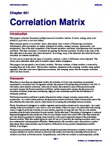
Fig. 1. Hybrid CRB (normalized with respect to the channel norm) versus temporal correlation coefficient ρ for different values of the SNR and K (M = 8, r = 3).
on N ). It follows that R = σ 2n /σ 2x IM . For simplicity, temporal correlation of the parameters is generated according to an autoregressive model of first order with ϕm = ρm , or equivalently matrix Rt has a Toeplitz structure with first column [1 ρ ρ2 · · · ρK−1 ]T , |ρ| ≤ 1. The behavior of the lower bound (trace of HCRB in (18)) is shown in fig. 1 (normalized with respect to the norm E[||hk ||2 ]) versus the temporal correlation coefficient ρ for different values of the signal to noise ratio SN R = σ2x /σ 2n and K. Larger values of ρ make temporal filtering of the parameters more effective and accordingly the HCRB decreases. As expected, this is increasingly true for a larger observation interval K, most noticeably for low SNR’s. The MSE of the proposed estimator M SEhˆ = ˆ − h||2 ]/K versus SNR (ρ = 0.8) for varying number of E[||h blocks (K) is in fig. 2. Notice from fig. 1 that the HCRB for ρ = 0.8 is essentially independent on K so that fig. 2 shows only the HCRB (dashed lines) for K = 100 (as for others K values it would be similar). According to the consistency of ˆ h , the hybrid estimator reaches the MoM for the estimate R the HCRB for large K and SN R. VI. C ONCLUSION The considered time-varying channel model for estimation of block-fading channels is quite general as the channel vector is modelled as a stationary Gaussian process with unknown and generally rank-deficient correlation matrix. The model applies to single and multi-antennas with appropriate definitions of the parameters into play. The proposed method approaches the estimate of the mixing deterministic/stochastic terms by decoupling the estimation of stationary rank-deficient correlation with the Method of Moments and the time-varying fading with the MMSE principle. Moreover, a bound on the estimation error has been derived though calculation of the Hybrid CRB. The numerical analysis has proved that the
10
-10
-5
0
5
10 SNR [dB]
15
20
25
30
Fig. 2. MSE of the proposed estimator versus SNR for different values of K (M = 8, r = 3, ρ = 0.8).
hybrid estimator is asymptotically efficient with the number of blocks. VII. A PPENDIX : PROOF OF EQUALITY (18) From the matrix inversion lemma: (D−1 +FE−1 FH )
−1
= D − DF(E + FH DF)−1 FH DH (21) given invertible matrices D and E and matrix F with appro−1 priate dimensions. The term [J]bb = (IK ⊗CAH R−1 ACH + −1 −1 Rt ⊗ IM ) in the right hand side of first form of eq.(18) can be cast into a form suitable for the application of (21) by defining D = Rt ⊗ IM , E = IK ⊗ R and F = IK ⊗ CAH . Now, using (21) and usual properties of the Kronecker product, second form of eq.(18) is easily obtained. R EFERENCES [1] E. Biglieri, J. Proakis and S. Shamai, ”Fading channels: informationtheoretic and communications aspects,” IEEE Trans. Inform. Theory, vol. 44, no. 6, pp. 2619-2692, Oct. 1998. [2] F.A. Dietrich, W. Utschick, ”Pilot-assisted channel estimation based on second-order statistics,” IEEE Trans. Signal Processing, vol.53, no. 3, pp.1178-1193, March 2005. [3] P. Stoica and M. Viberg, ”Maximum likelihood parameter and rank estimation in reduced-rank multivariate regressions,” IEEE Trans. Signal Processing, vol. 44, no. 12, pp. 3069-3078, Dec. 1996. [4] M. Nicoli and U. Spagnolini, ”Reduced-rank channel estimation for timeslotted mobile communication systems,” IEEE Trans. Signal Processing, vol. 53, no. 3, pp. 926-944, March 2005. [5] O. Edfors, M. Sandell, J.-J. van de Beek, S. K. Wilson, P .O. Borjesson, ”OFDM channel estimation by singular value decomposition,” IEEE Trans. Commun., vol. 46, no. 7, pp. 931-939, July 1998. [6] D. Shiu, G. J. Foschini and M. J. Gans, ”Fading correlation and its effect on the capacity of multielement antenna systems,” IEEE Trans. Commun., vol. 48, no. 3, March 2000. [7] H. L. Van Trees, Optimum array processing, J. Wiley Ed. 2002. [8] O. Simeone and U. Spagnolini, ”Lower bound on training-based channel estimation error for frequency-selective block-fading Rayleigh MIMO channels,” IEEE Trans. Signal Processing, vol. 52, no. 11, pp. 3265-3277, Nov. 2004. [9] P. Stoica and T. L. Marzetta, ”Parameter estimation problem with singular information matrices,” IEEE Trans. Signal Processing, vol. 49, no. 1, pp. 87-90, Jan. 2001.