Estimation of Spatial Weights Matrix, with an Application to Diffusion in Housing Demand Arnab Bhattacharjee and Chris Jensen-Butler School of Economics and Finance University of St. Andrews, UK.
∗
May 1, 2006
Abstract While estimates of models with spatial interaction are very sensitive to the choice of spatial weights, considerable uncertainty surrounds definition of spatial weights in most studies with cross-section dependence. We propose a new methodology for estimation of spatial weights matrices in the spatial error model, which are consistent with an observed pattern of spatial autocovariances. The estimated spatial weights are useful for identifying the real rather than hypothesised determinants of spatial interaction. The methodology is applied to regional housing markets in the UK, providing an estimated spatial weights matrix that generates several new hypotheses about the economic and socio-cultural drivers of spatial diffusion in housing demand.
Keywords: Spatial econometrics; Spatial autocorrelation; Spatial weights matrix, Spatial error model; Housing demand; Gradient projection. JEL Classification: C14; C15; C30; C31; R21; R31. ∗
Corresponding author: A. Bhattacharjee, School of Economics and Finance, University of St. Andrews, Castlecliffe, The Scores, St. Andrews KY16 9AL, UK. Tel: +44 1334 462423. e-mail:
[email protected] We thank Tatiana Damjanovic, Donald Haurin and Geoff Meen for helpful suggestions on the work. We also thank Hometrack and particularly David Catt and Richard Donnell for access to part of the data used in this paper. The usual disclaimer applies.
1
1
Introduction
The usual approach to the representation of spatial dependence in econometric studies is to define a spatial weights matrix, which represents a theoretical and a priori understanding of the nature of spatial interdependence between different geographical regions or, more generally, between different economic agents. These spatial weights represent patterns of interaction and diffusion, and thereby provide a meaningful and easily interpretable representation of spatial interaction (spatial autocorrelation) in spatial dependence models. In combination with spatial structure (spatial heterogeneity), they offer a useful framework for studying cross-sectional dependence (see, for example, Anselin, 1988, 1999). The spatial weights are usually interpreted as functions of relevant measures of economic or geographic distance (Anselin, 1988, 2002). The distance between two agents reflects their proximity with respect to unobservables, so that the joint distribution of random variables at a set of points can be represented as a function of the economic distances between them. The choice of appropriate spatial weights is a central component of spatial models as it imposes a priori a structure of spatial dependence, which may or may not correspond to reality. Further, the accuracy of these measures affects profoundly the estimation of spatial dependence models (Anselin, 2002; Fingleton, 2003). The choice typically differs widely across applications, depending not only on the specific economic context but also on availability of data. Spatial contiguity (resting upon implicit assumptions about contagious processes) using a binary representation, is a frequent choice. Further, in many applications, there are multiple possible choices and substantial uncertainty regarding the appropriate choice of distance measures. However, while existing literature contains an implicit acknowledgment of these issues, most empirical studies treat spatial (and spmetimes spatio-temporal) dependence in a superficial manner assuming inflexible diffusion processes in terms of known, fixed and arbitrary spatial weights matrices (Giacomini and Granger, 2004). The problem of choosing spatial weights becomes a key issue in many economic applications1 . However, the spatial econometrics literature tells us little about adequate foundations for these choices. Acknowledging the uncertainty regarding specification of economic distances in most applications using spatial models, 1
Ethnic networks and trade, spatial demand for goods and services, risk-sharing in rural developing economies, and convergence in growth models, to name only a few (see Conley, 1999; Fingleton, 2003; Herander and Saavedra, 2005). Similar issues regarding the choice of spatial weights have also been addressed in the regional science and urban economics literature (Lacombe, 2004; Aten and Heston, 2005).
2
Conley (1999) proposed a strategy allowing for imperfectly measured economic distances and used these distances to obtain asymptotic estimators of the implied spatial autocovariance matrices. Pinkse et al. (2002) develop a framework which accommodates uncertainty regarding distance measures and allows for spatial nonstationarity; related work is developed in Kelejian and Prucha (2004). In this paper, we take a different nonparametric view on the nature and strength of spatial diffusion. As a new departure from the literature, we develop a method for estimating spatial weights matrices that are consistent with an observed pattern of spatial (or cross sectional) dependence. Once these spatial weights have been estimated they can be subjected to interpretation in order to identify the true nature of spatial dependence, representing a significant departure from the usual practice of assuming a priori the nature of spatial interactions. The approach developed here builds upon the spatial error model with autoregressive errors, but is, however, extendable to other models of spatial dependence. An illustration of the proposed methodology and its potential is presented in the paper through a model-based study of regional housing markets in England and Wales, where the aim is to identify the economic and sociocultural drivers of spatial diffusion in housing demand. Whilst the study of spatial diffusion of demand in the housing market is in itself not new (for example, in the case of the UK: Meen, 2001, 2003; and for the US: Haurin and Brasington, 1996; Fik et al., 2003), the ex post approach to identifying drivers of diffusion presented here is novel and some of the results are both surprising and not explainable by simple contiguity assumptions. Section 2 describes the econometric framework and the methodology for estimation of the spatial weights matrix. In section 3, we discuss asymptotic properties of the estimator, bootstrap estimation of standard errors and hypothesis tests. Results of a Monte Carlo simulation study calibrated to the Barro and Sala-i-Martin (1992) study of β-convergence across census divisions in the US are reported in section 4. In section 5, we apply our methods to the study of spatial diffusion in housing demand in England and Wales and section 6 draws together the conclusions.
2
Proposed Estimation Methodology
In this section, we propose methods for estimation of the spatial weights matrix when spatial dependence is in the form of a spatial error model. Much 3
of our discussion is in the context of a model where the error process of spatial diffusion has an autoregressive structure; the extension of the methods to a moving average spatial error model is straightforward. The proposed estimates are constructed using a consistent estimate of the spatial autocovariance matrix. In the following subsections, we first present our econometric model of spatial diffusion, along with the assumptions. Next, we discuss estimation of the spatial weights matrix implied by the given (estimated) autocovariance matrix of the spatial errors. Finally, we review the existing literature on estimation of the spatial autocovariance matrix under different model assumptions.
2.1
The Spatial Error Model
Studies in spatial econometrics typically distinguish between two different kinds of spatial effects in regression models for cross-sectional and panel data — spatial interaction (spatial autocorrelation) and spatial structure (spatial heterogeneity). While the study of spatial structure is similar to the traditional treatment of coefficient heterogeneity in econometrics, spatial interaction is usually modeled through a pre-determined spatial weights matrix. The problems associated with prespecified spatial weights matrices are wellknown: the choice of weights is frequently arbitrary, there is substantial uncertainty regarding the choice, and the results from studies vary considerably according to the choice of spatial weights. Given a particular choice of the spatial weights matrix, there are two important and distinct ways in which spatial interaction is modelled in spatial regression analysis — the spatial error model (SEM) and the spatial lag model (SLM). In the following discussion, we focus on regional demand in housing — consistent with an application presented later in the paper. The applicability of the model and the methodology are, however, not in any way specific to this application. We consider panel data on demand and other explanatory variables across various regions over several time periods. Within the context of estimated demand equations for each of several regions, we aim to understand how excess demand in any region diffuses over space to the other regions. Regional demand (D) is modeled using a simple structural spatial error model, where is explained by the effects of explanatory variables (X) and diffusion of excess demand from other regions. The spatial externalities in the form of demand diffusion are driven by the completely unspecified pattern of spatial weights (given by the spatial weights matrix W ) and the strength of spatial spillovers in each region described by spatial autocorrelation para-
4
meters ρK . The model and its reduced form are described as follows: Dt ut
= X t .β + ut , t = 1, . . . , T, = R.W .ut + εt , =⇒ Dt = X t .β + (I − R.W )−1 .εt ,
(1)
where there are T time periods (t = 1, . . . , T ) and K regions (k = 1, . . . , K), Dt is the K × 1 vector of regional demand in period t, W is an unknown spatial weights matrix of dimension K × K, R = diag (ρ1 , ρ2 , . . . , ρK ) is a K ×K diagonal matrix containing the (possibly heterogeneous) spatial autoregression parameters for each region2 , and εt is the K × 1 vector of independent but possibly heteroscedastic spatial errors. In this model, the spatial diffusion of errors is assumed to be autoregressive; we call this model the spatial error model with autoregressive errors (SEM-AR). The spatial diffusion of errors can also be modelled as a moving average process (Anselin, 1988), where we have the spatial error model with moving average errors (SEM-MA): ut
= R.W .εt + εt , =⇒ Dt = X t .β + (I + R.W ) .εt .
(2)
The above formulation of the SEM-AR and SEM-MA models represent several departures from the literature. First and foremost, we do not assume a given form of the spatial weights matrix. Indeed, our aim is to estimate the spatial weights matrix implied by the observed pattern of spatial autocorrelations (autocovariances). Second, we allow the spatial autoregression (spillover) parameters to vary across agents or regions, and also to be unknown. This flexibility in spatial spillovers captures an important dimension of heterogeneity. Third, the description of the model also allows for heterogeneity in the regressors as well as their coefficients across the regions, a feature which is important in the application considered later. Fourth, we allow heteroscedasticity in the errors across regions. However, all spatial autocorrelation under the model is completely specified by the spatial weights matrix and the spatial autoregression parameters. This is the 2 ⎞ in the paper, diag(a1 , a2 , . . . , ak ) denotes the diagonal matrix ⎛ Here, and henceforth a1 0 . . . 0 ⎜ 0 a2 . . . 0 ⎟ ⎟ ⎜ ⎜ .. .. . . .. ⎟. ⎝ . . . . ⎠
0
0
. . . aK
5
crucial feature in the model that allows us to estimate the implied spatial weights from the observed spatial autocovariances. Simple types of temporal variation, such as those in the nature of simple autoregressive or moving average processes in the temporal dimension, can also be easily accommodated in our framework. However, for reasons of expositional simplicity, we abstract from the issue of temporal dynamics in this paper. In other words, we assume independence of the joint distribution of the variables over time, but not over space. An alternative model considered in the literature is the spatial lag model (Anselin, 1988). A prominent example is the mixed regressive spatial autoregressive model (Ord, 1975) described as: Dt = R.W .Dt + X t .β + εt , t = 1, . . . , T, ⇒ Dt = (I − R.W )−1 .X t .β + (I − R.W )−1 .εt .
(3)
The choice between the spatial error model and the spatial lag model is largely context specific and often quite difficult. Though different in interpretation, the two kinds of models are difficult to distinguish empirically (Anselin, 1999, 2002). Based on a given spatial weights matrix, there are tests that can help decide between the two models3 . In this paper, we focus on the spatial error model with autoregressive errors (Equation 1). From the point of view of relevant theory in housing economics, we find this model well suited to explain housing demand in terms of spatial diffusion of excess demand from neighbouring regions, where neighbourhood is defined in an abstract sense. We also discuss the spatial error model with moving average errors (Equation 2). While similar analysis of other spatial interaction models is left to future work, we make some comments regarding these models later in the paper. The above discussion is formalised in the following assumptions. Assumption 1: We assume that the spatial errors, εt , are iid (independent and identically distributed) across for het¡ time. ¢ However, we 2allow T 2 eroscedasticity across regions, so that E εt .εt = Σ = diag (σ1 , σ 2 , . . . , σ 2K ), and σ 2k > 0 for all k = 1, . . . , K 4 . The uncorrelatedness of the spatial errors across the regions is the crucial assumption in this paper. Assumption 1 ensures that all spatial autocorrelation in the model is solely due to spatial diffusion described by the spatial 3
See Anselin (2001) and Baltagi et al. (2003) for reviews of tests designed to aid model choice. 4 Here and throughout the paper, T denotes transpose of a vector or matrix.
6
weights matrix and the autoregression coefficients; this feature of the model drives our estimation strategy. Assumption 2: The spatial weights matrix W is unknown and possibly asymmetric. W has zero diagonal elements and there are no restrictions on the off-diagonal elements (i.e., they could be either positive or negative). As discussed in the previous section, the literature on spatial modelling acknowledges substantial uncertainty in the specification of appropriate spatial weights. Practitioners are usually encouraged to exercise caution in the choice of the spatial weights matrix, and also to experiment with different choices. If the spatial weights are inversely related to some underlying metric distance between the regions, then the spatial weights matrix would typically be symmetric. At the moment, we retain the flexibility of a possibly asymmetric spatial weights matrix, though symmetry is assumed subsequently (Assumption 5). Our most significant point of departure from the literature is in the assumption of an unknown spatial weights matrix, and we propose a methodology for its estimation. We do not impose a non-negativity constraint on the off-diagonal elements of W ; later we discuss situations when negative off-diagonal elements may be expected. In fact, in an application related to ours, Meen (1996) finds evidence of negative interaction between various regions. We will show that the spatial weights matrix is identified by the spatial autocovariance matrix only upto an orthogonal transformation, except under rather restrictive conditions. Additional assumptions, such as symmetry of the spatial weights matrix, homoscedasticity or row-standardisation, are required for the estimation of spatial weights in general. Assumption 3: (I − R.W ) is non-singular, where I is the identity matrix. This is a standard assumption in the literature Under Assumption 3, the reduced form representation of the SEM-AR model (Equation 1) is given by: Dt = X t .β + ut = X t .β + (I − R.W )−1 .εt , where (dropping the time subscript) ¢ ¡ T E u.uT = (I − R.W )−1 .Σ. (I − R.W )−1 . 7
Assumption 4: For the SEM-AR ¡ ¢ model (Equation 1), the population spatial autocovariance matrix, E u.uT , is unknown and positive definite with probability one, but otherwise has a completely unrestricted structure. Furb of the population spatial autocother, there exists a ¡consistent estimator, Γ, ¢ T variance matrix E u.u . b We assume that this structural model can be estimated, and ¡ letT ¢Γ denote a consistent estimator of the spatial autocovariance matrix E u.u . Below, b to estimate the implied spatial weights we describe a method that uses Γ matrix.
2.2
Estimation of Spatial Weights
Meen (1996) studies spatial diffusion in housing starts across regions in England under a SEM-AR model by regressing OLS residuals of the regression relationship for each region on residuals from all the other regions Dt = X t .β + ut , (First step regression) b u b = X t .β, t
u bkt = ρk .
K X
wkj .b ujt + εkt , (Second step regressions)
(4)
j=1 j6=k
where the second step regressions are run separately for each region5 . The sign and statistical significance of the OLS regression estimates at the second step are used to examine the potential importance of spatial dependence across the regions. This approach can be described as a first attempt towards estimating the unknown spatial weights matrix up to a factor of proportionality (the spatial autoregressive parameter). This method, however, suffers from several limitations. First, under the SEM-AR model, the OLS estimates of the regression parameters of the original equation are consistent but inefficient. This inefficiency directly affects the estimates of the residuals from the regression in the first step, and therefore affects the second step regression using these 5
Note that, Meen (1996) assumes homogeneity in the spatial autoregression parameter across the regions. For expositional clarity, we retain heterogeneity in the spatial autoregression parameter at this stage. However, we impose homogeneity later on (Assumption 5), and in any case, the autoregression parameter is not separately identifiable from the estimate of the spatial weights matrix.
8
residuals. This problem can be resolved by using more appropriate estimation methods at the first step. Depending on the model framework and the chosen application, one could use seemingly unrelated regressions, two stage least squares or three stage least squares to estimate the first step regression. Second, and most importantly, the regressions on the residuals suffer from the serious problem of endogeneity, and therefore bias and inconsistency of the estimates of regression coefficients. Third, the second step involves estimating regressions through the origin, and hence the results have to be interpreted appropriately. Fourth, there is no simple way to extend this method to estimation of spatial weights in other models of spatial interaction. Our proposed estimation method is somewhat similar to Meen (1996), to the extent that we too start by estimating the first step regression equation. However, at the second step we do not explicitly regress the residuals from the first step, but use the reduced form of the second step regression to estimate the spatial weights matrix (up to a factor of proportionality) directly from the spatial autocovariance matrix estimated in the first step. Note that the error covariance matrix, Σ = diag (σ21 , σ 22 , . . . , σ 2K ), of the structural equations is diagonal (Assumption 1), implying that all spatial autocorrelation in the model arises from the spatial weights matrix W , while allowing for heteroscedasticity between the spatial units. Our method for consistent estimation of the spatial weights matrix relies on the structure of the problem: most importantly, the zero diagonal elements of the spatial weights matrix (Assumption ¡ T ¢ 2) and the diagonal structure of the covariance matrix (Σ = E ε.ε ) of the spatial errors (Assumption 1). The proposed method is assumption-free, in the sense that it is completely based b and does not a priori on an estimate of the spatial autocovariance matrix, Γ, impose any structure on the drivers of spatial diffusion. ¡ ¢ Let Γ = E.Λ.E T denote the eigenvalue decomposition of Γ = E u.uT , where Λ = diag (λ1 , λ2 , . . . , λK ) is the diagonal matrix of eigenvalues and the columns of E = [e1 , e2 , . . . , eK ] contain the corresponding eigenvectors. Proposition 1 Let Assumptions 1—4 hold. Then, upto an orthogonal transformation, the matrix ¶ µ 1 1 1 T V = (I − R.W ) .diag (5) , ,..., σ1 σ2 σK b−1/2 = E. b Λ b −1/2 .E b T , where E b and Λ b contain is consistently estimated by Γ the eigenvectors and eigenvalues respectively of the estimated spatial autob In other words, Γ b−1/2 is a consistent estimator of covariance matrix Γ. 9
V.T for some unknown square orthogonal matrix T . Further, if the rows b−1/2 is a consistent estiof (I − R.W ) are orthogonal to each other, then Γ mator of V . Proof. First, consider the spectral decomposition of Γ−1 , Γ−1 = (I − R.W )T .Σ−1 . (I − R.W ) = V .V T .
(6)
This implies that Γ−1 = (V .T ) . (V .T )T , for any square orthogonal matrix T . Next, consider the eigenvalue decomposition of the consistent estimated cob variance matrix Γ: b = E. b Λ. bE bT, Γ (7)
b b = diag (λ1 , λ2 , . . . , λK ) is the diagonal matrix of eigenvalues of Γ, where Λ b and the columns of E = [e1 , e2 , . . . , eK ] contain the corresponding eigenvectors. b is positive definite with probability one (Assumption 4), Note that, since Γ min (λ1 , λ2 , . . . , λK ) > 0 with probability one and ¶ µ −1/2 1 1 1 b . = diag √ , √ , . . . , √ Λ λ1 λ2 λK Therefore, from Equation (7) it follows that, the eigenvalue decomposition of b −1 is given by: Γ b −1 = E.Λ−1 .E T Γ = E.Λ−1/2 .E T .E.Λ−1/2 .E T ´ ³ ´T ³ −1/2 T −1/2 T = E.Λ .E . E.Λ .E .
(8)
The first step holds because E −1 = E T , and the final step follows since Λ−1/2 is a symmetric matrix. From Equations (6) and (8), the matrix V can be consistently estimated,
10
upto an orthogonal transformation, by Vb
b Λ b −1/2 .E bT = E. ¶ µ 1 1 1 bT b √ , √ ,..., √ .E = E.diag λ1 λ2 λK 1 1 1 = √ e1 eT1 + √ e2 eT2 + . . . + √ eK eTK λ λ2 λK ⎛ 1 ⎞ vb11 vb12 . . . vb1K ⎜ vb21 vb22 . . . vb2K ⎟ ⎜ ⎟ = ⎜ .. .. . . .. ⎟ , ⎝ . . . . ⎠ vbK1 vbK2 . . . vbKK
(9)
where we denote the elements of the matrix Vb by vbij (i, j = 1, . . . , K). If the rows of (I − R.W ) are orthogonal to each other, then the spectral decomposition of Γ−1 is unique and T is the identity matrix; hence, exact equivalence holds. Since the rows of (I − R.W ) are orthogonal only in special cases6 , the above Propositition is not very useful in itself. In the following arguments, we develop additional assumptions under which the orthogonal matrix T can be uniquely identified. Assumption 5: The spatial weights matrix is symmetric and the spatial autoregression parameter is the same across all regions; in other words R.W = ρW is symmetric. Note that symmetry of the spatial weights matrix can be a strong assumption in some applied situations. Row-standardised spatial weights matrices are usually asymmetric by construction; asymmetric spatial weights matrices are also important in the study of asymmetric shocks, network flows and core-periphery models. Later, we discuss alternative sets of assumptions that may be useful in such situations. Proposition 2 Let Assumptions 1—4 hold. Then, there exists a unique orthogonal matrix T for which Assumption 5 also holds. Proof. Under Assumption 5, we can express Equation (5) as: ¶ µ 1 1 1 T V = (I − R.W ) .diag , ,..., σ1 σ2 σK ¶ µ 1 1 1 T . , ,..., = (I − ρ.W ) .diag σ1 σ2 σK 6
Such as, when the spatial weights matrix is zero.
11
Therefore, what the Proposition says is that given any positive definite Γ−1/2 , there exists a unique orthogonal matrix T such that the matrix ¶¸ ∙ µ 1 1 1 T −1/2 Γ .T T = (I − ρ.W ) .diag , ,..., σ1 σ2 σK is symmetric. The above expression can be rewritten as: ¶¸ ∙ µ 1 1 1 T −1/2 .T = (I − ρ.W ) .diag , ,..., Γ σ1 σ2 σK = Q = ((qij ))i,j=1,...,K . Now, since (a) post-multiplication by the diagonal matrix diag
³
1 , 1 , . . . , σ1K σ1 σ2
´
transforms (I − ρ.W )T by multiplying each column by the corresponding diagonal element, and (b) by Assumption 3, the elements on the diagonal of (I − ρ.W )T are all unity, we have ⎡ ⎤ 1 q12 /q11 . . . q1K /q11 ⎢ q21 /q22 1 . . . q2K /q22 ⎥ ⎢ ⎥ T (I − ρ.W ) = ⎢ ⎥. .. .. .. . . ⎣ ⎦ . . . . 1 qK1 /qKK qK2 /qKK . . .
Therefore, the condition that the spatial weights matrix is symmetric (Assumption 5) implies that qij qji = , for all i 6= j; i, j = 1, . . . , K. qii qjj
(10)
Further, note that T consists of K 2 real values, and several restrictions apply to the elements of this matrix. Specifically, there are K normalization restrictions (one for each column of the matrix) and K(K − 1)/2 orthogonality conditions (one for each distinct pair of columns). This leaves K 2 − [K + K(K − 1)/2] = K(K − 1)/2 free elements in the matrix. These free elements can be pinned down by the K(K − 1)/2 constraints relating to the assumption of symmetry (Equation 10). This identification is upto a sign transformation on the columns and rows of T that preserves the orthogonality condition while at the same time ensuring that the diagonal elements of the transformed matrix are all positive. The identification and uniqueness of T can be easily verified for the 2-region case, where any orthogonal matrix can be written as ∙ ¸ cos φ − sin φ . sin φ cos φ 12
The proof in the general case is quite involved and not elaborated on. The condition can be numerically verified quite easily for any given Γ. Of course, there can be many different ways sets of constraints that would pin down the orthogonal matrix T . In fact, one need not even explicitly specify the constraints. Jennrich (2001) has recently proposed a “gradient projection” algorithm for optimising any objective function over the group of orthogonal transformations of a given matrix. The only conditions necessary for implementing the algorithm are that (a) the objective function is differentiable, and (b) there exists a stationary point of the objective function within the class of orthogonal transformations. Here, we adapt this algorithm to our case. For the estimated Vb and any orthogonal matrix T , define (i) a matrix Q = Vb .T = ((qij ))i,j=1,...,K ,
(11)
(ii) a scalar function of T (our objective function): f (T ) =
K−1 X i=1
¶2 K µ X qij qji − , qii qjj j=i+1
(12)
(iii) a gradient matrix df dT where gii
gij
T = Vb .G; G = ((gij ))i,j=1,...,K , ¸ ∙ K 2 X qik qki = − 2. qik . − qii k=1 qii qkk
∙
k6=i
2 qij qji = . − qii qii qjj
¸
(13)
if i 6= j.
and (iv) a scalar constant ° ¢° ¡ (14) s = °skm T T .G ° , ¢ ¡ ¢ ¡ where skm(B) = 12 B − B T and kBk = tr B T .B denote the skew symmetric part and the Frobenius norm respectively of a square matrix B.
13
Algorithm: Choose α > 0 and a small ε > 0, and set T to some arbitrary initial orthogonal matrix7 . (a) Compute s. If s < ε, stop. (b) Compute G. e = (c) Find the singular value decomposition A.D.C T of T − α.G; set T T A.C . e . If any diagonal element of Q is negative, multiply (d) Compute Q = Vb .T e by −1. the corresponding column of T e (e) If f (T ) ≥ f (T ), replace α by ´i ¡ ¢ h ³ e ) − f (T ) + s2 .α α e = s2 .α2 / 2. f (T e ) < f (T ), replace T by T e and go to (a). and go to (c). If f (T
b , is such that all diagonal elements The estimate of T at convergence, T of the matrix b = Vb .T b = ((b Q qij )) i,j=1,...,K
b , the spatial error variances can be estimated as are positive. Given this T σ b2k =
1 , k = 1, . . . , K qbii2
and the spatial weights matrix as: ⎡ 0 −b q21 /b q22 ⎢ −b q12 /b q11 0 d =⎢ ρW ⎢ .. .. ⎣ . . q11 −b q2K /b q22 −b q1K /b
. . . −b qK1 /b qKK . . . −b qK2 /b qKK .. ... . ... 0
(15)
⎤
⎥ ⎥ ⎥. ⎦
(16)
Proposition 3 The algorithm is strictly monotone and stops when it is sufficiently close to a stationary point. The return to step (c) from (e) occurs only a finite number of times. b , of the relevant orthogonal Under Assumptions 1—5, the final estimate, T b matrix is such that Q has positive diagonal elements, and the estimated spad , is symmetric. tial weights matrix, ρW 2 d σ bk and ρW are consistent estimators of the respective parameters of the model (Equation 1). 7
We choose a set of random orthogonal matrices, including the identity matrix, to ensure that the algorithm does not get stuck up in a local stationary point that does not optimise the objective function.
14
Proof. Note that, reversing the sign of each element in a specific column of T reverses the sign of the corresponding diagonal element of Q = Vb .T , but preserves the orthogonality of T . Therefore, step (d) ensures that the diagonal elements of Q are positive in each iteration of the algorithm. Effectively, our objective function is f (T ) =
K−1 X i=1
¶2 K µ X qij qji − , |q | |q | ii jj j=i+1
which is not a differentiable function when Q has any zero diagonal element. However, by Assumption 1 the spatial errors have positive variances, min (σ 21 , σ 22 , . . . , σ 2K ) > 0, and therefore in large samples the diagonal elements of Q will be away from zero8 . Therefore, close to each candidate T , f (.) is locally a smooth differentiable function of T which is bounded below by zero. Hence, a stationary point always exists. It can be verified easily that G = df/dT . Following arguments in Jennrich (2001), for sufficiently large α, the algorithm is convergent from any starting value and is expected to converge to a stationary point of f (.) over the group d is a of all orthogonal matrices. Therefore, σ b2k > 0 for k = 1, . . . , K and ρW symmetric matrix. Further, as discussed in the context of Proposition 2, the value at the stab = Vb .T b is a consistent estimator for tionary point is zero. Q h ³ Therefore,´i (I − ρ.W )T .diag σ11 , σ12 , . . . , σ1K . Note that, since the spatial weights matrix W has zero diagonal elements (Assumption 3), the elements on the diagonal of (I − ρ.W ) must all be b unity. Hence, under the model assumptions, the diagonal elements of Q are equal to σ11 , σ12 , . . . , σ1K respectively. From consistency of the spatial covariance matrix and by Proposition 1, it follows that σ b2k , k = 1 . . . , K are d is a consisconsistent estimators for σ 21 , σ 22 , . . . , σ 2K . It also follows that ρW tent estimator for the unknown and unrestricted spatial weights matrix ρW under Assumptions 1—5. The algorithm is simple to implement; there are, however, two important issues in the implementation. First, in principle, the choice of α can be quite critical. If α is too large, the convergence is very slow; on the other hand, if α is too small, there will be many returns to step (c) from step (e). However, 8
This argument can be made more precise by imposing a boundedness assumption on the spatial error variances.
15
in practice this does not turn out to be a problem9 . Second, there might be a problem with the implementation if Step (d) is implemented too many times. This would mean that we are starting too far from the stationary point, and every time that one of the negative diagonal elements of Q is corrected for, we are moving away from the stationary point instead of taking an optimal step along the gradient; this does not turn out to be an important issue in our implementation. The assumption of a symmetric spatial weights matrix (Assumption 5) may be too restrictive in many applications. First, it is often convenient to work with row-standardised spatial weights matrices (Anselin, 1999), which are asymmetric by construction. Second, there are applications where it is reasonable to expect asymmetric strength of diffusion between regions. For example, the strength of diffusion from a spatial unit on the periphery to the core may well be different from that from the core to the peripheral region. Third, if we do not assume homogeneity in the autoregression parameter ρk across the regions, the matrix R.W will be asymmetric; such heterogeneity may be quite natural in many situations, like in a core-periphery structure or in relation to flows in a network. However, the framework developed here is flexible and can admit many other sets of conditions. Useful constraints in this context could include setting the row sums of the estimated spatial weights matrix equal to each other10 , or homoscedasticity in all or some of the spatial error variances, or constraints on specific spatial autocorrelations, or even a combination of several constaints. For example, in an application with 4 regions, we would require 6 constraints: 3 of these constraints can come from the homoscedasticity assumption, while the remaining 3 can be obtained by restricting to row-standardised spatial weights matrices. Further, note that, setting the constraints is not essential for implementing the gradient projection algorithm. What one requires is a suitable objective function to optimise; this objective function should be differentiable and should have a stationary point within the class of orthogonal rotations. Instead of the objective function used here (Equation 12), one could use variance of diagonal elements or of row-sums as alternative optimisation criteria. Similarly, some of the optimisation criteria commonly used in factor analysis could be useful in some spatial applications11 . 9
In our implementation, we did some trial and error to choose an optimal α before starting the iterations. Once this choice was made, the convergence was very fast in about 95 per cent of the cases. 10 This would be relevant when all spatial weights are positive and one is interested in estimating the row standardised spatial weights matrix. 11 See Jennrich (2001) for discussion on several optimisation criteria (quartimax, or-
16
d (or in the more general case, A notable feature of our estimator ρW when Assumption 5 is not imposed, R.W ) is that the covariance pattern in the errors is determined solely by the product R.W . This observation has implications for the estimation of the spatial weights. A property of this estimator, which derives from the underlying spatial error model, is that the autoregression parameters ρk are in general not identifiable separately from the spatial weights matrix W , so that only the product R.W is usually estimable, and not the individual components R and W . Note, however, that the row-standardised spatial weights matrix, W (RS) , can be uniquely estimated as: ⎛ # # ⎞ "K "K X X ⎟ ⎜ 0 qb21 / . . . qbK1 / qbk1 qbk1 ⎟ ⎜ k=2 k=2 ⎟ ⎜ ⎤ ⎤ ⎡ ⎡ ⎟ ⎜ K K X X ⎟ ⎜ ⎜ qb12 / ⎣ qbk2 ⎦ qbk2 ⎦ ⎟ 0 . . . qbK2 / ⎣ (RS) ⎟ ⎜ c W =⎜ ⎟ k=1,k6 = 2 k=1,k6 = 2 ⎟ ⎜ ⎟ ⎜ .. .. .. ... ⎟ ⎜ . . . ⎟ ⎜ # # "K−1 "K−1 ⎟ ⎜ X X ⎠ ⎝ qb / qb / ... 0 qb qb kK
1K
kK
2K
k=1
k=1
(17) Further, R.W is obtained by premultiplying the spatial weights matrix by a diagonal matrix whose diagonal elements are the spatial autoregressive parameters for each region. Hence, the estimates of the spatial autoregressive parameters corresponding to the above row-standardised spatial weights matrix are given by: (RS) b ρk
=
K X
l=1,l6=k
qblk , k = 1, . . . , K.
(18)
As mentioned earlier, there is one other interesting feature of the estimator described here. It is possible that some of the estimated spatial weights d may be negative. This happens if qbij > 0 for some i 6= j. When the in ρW underlying spatial weights matrix has positive off-diagonal elements, we can have negative estimates of spatial weights because of sampling variations. thomax, etc.), and on extensions of the algorithm. If the objective function is complicated, deriving an analytic expression for the gradient can become difficult. However, in this case, one can replace the analytical gradients used in the algorithm by numerical derivatives (Jennrich, 2004).
17
However, spatial weights can be negative even in other situations. For example, in the context of housing demand across regions, such negative weights would imply that the excess demand in the index region is negatively related to some of the other regions. This can happen because of asynchronicity of the underlying housing market cycles in these regions, as would be expected for example if there are ripple effects (Meen, 1999), or if the two regions provide substitute housing markets. Meen (1996) explains negative interaction between regions in a study of housing starts as arising from planning restrictions in certain regions Under the spatial error model with moving average errors (Equation 2), the spatial weights matrix can be consistently estimated in a very similar manner. In this model, the spatial autocovariance matrix is given by: ¡ ¢ Γ = E u.uT = (I + R.W ) .Σ. (I + R.W )T = Z.Z T = (Z.T ) . (Z.T )T ,
where Z = (I + R.W ) .diag (σ1 , σ 2 , . . . , σ K ) , and T is any orthogonal matrix. Therefore, under the symmetric spatial b exactly in the weights matrix assumption (Assumption 5), we estimate Q same way as the SEM-AR model. The estimator for the spatial weights matrix is now given by: ⎡ ⎤ 0 qb21 /b q22 . . . qbK1 /b qKK ⎢ qb12 /b q11 0 . . . qbK2 /b qKK ⎥ ⎥ d (MA) = ⎢ (19) ρW ⎢ ⎥. .. .. .. ... ⎣ ⎦ . . . q11 qb2K /b q22 . . . 0 qb1K /b
Estimation of the spatial weights matrix for the spatial lag model (Equation 3) turns out to be a more difficult problem. This is because, the spatial weights matrix enters the reduced form of the model through the spatial filter, (I − R.W )−1 , applied to both the regressors and the spatial errors. Given sufficient data, one can estimate the spatial error autocovariance matrix using regressors for all the regions (except the index region) instead of the (unknown) filtered regressors. This estimated spatial autocovariance matrix can then be used to estimate the spatial weights matrix. However, this would give only a limited information estimator, since it does not exploit the additional information on the spatial weights embedded in the regression 18
coefficients. Similarly, an alternative limited information strategy could be extracting the information on the spatial weights from the regression coefficients. Finding a way to combine these two estimation methods requires further work.
2.3
Estimates of the Spatial Autocovariance Matrix
In the previous subsection, we developed consistent estimates of the spatial weights matrix based on a given consistent estimate of the spatial autocovariance function of regression errors. Here, we discuss estimation of the underlying spatial autocovariance matrix and implications for estimation of the spatial weights. When the regressors, X, included in the SEM-AR or SEM-MA model (Equations 1 and 2) are exogenous, Meen (1996) proposes estimation of the spatial autocovariance matrix using seemingly unrelated regressions (SURE). This procedure begins with initial nonparametric estimation of the spatial autocovariance matrix of reduced form errors (u) from a first stage regression, performs GLS-type estimation using this estimated covariance matrix, and continues iteration till convergence. As emphasized by Anselin (1999), the SURE approach is very general and does not require any specification of spatial processes or indeed any functional form for distance decay. Further, the procedure naturally allows estimation of a spatial regime model (Anselin, 2002) incorporating region-specific heterogeneity in slope, intercept and even the choice of regressors. Since the SURE estimator is a maximum likelihood estimator (MLE), the proposed estimator of the spatial weights matrix based on a spatial autocovariance matrix estimated using SURE will also be the MLE. Therefore, this estimator of the unknown spatial weights matrix will possess the desirable asymptotic properties of MLEs, including efficiency and asymptotic normality. If some of the regressors are endogenous, we can proceed as in the twostage least squares (2SLS) procedure by computing predictions of the endogenous variables by regressing them on the instruments. Next, we can use the residuals from the second-stage regression to estimate the spatial autocovariance matrix. Like SURE, one can iterate this process using GLS-type estimation, but this does not give efficiency gains. The resulting estimator is consistent, but will not be asymptotically efficient if the instruments are weak (Staiger and Stock, 1997) If we have a system of simultaneous equations involving the endogenous variables, efficiency gains can be made by allowing the covariances across the equations to be possibly non-zero. The parameters of the structural equation and the spatial autocovariance matrix can be estimated as in the earlier case, 19
using a three stage least squares (3SLS) procedure. The estimates can be iterated to convergence, but there are no asymptotic efficiency gains to the iterative procedure; the 3SLS estimator itself is asymptotically efficient and has asymptotic properties similar to the MLE.
3 3.1
Asymptotic Properties and Hypothesis Tests Consistency and Asymptotic Distribution
d (or R.W \ in the more general Asymptotic properties of our estimator ρW case) depend directly from the properties of the underlying spatial autocob Under the assumptions that the spatial errors have posvariance matrix Γ. itive variance (Assumption 1), (I − R.W ) is non-singular (Assumption d is a continuous 3) and the identification condition (Assumption 6), ρW b Similarly, W c (RS) function of the estimated spatial autocovariance matrix Γ. (RS) b Hence, and following arguments and b ρk are also continuous functions of Γ. in Proposition 3, these estimators are consistent for the underlying true spatial weights matrix and the region-specific autocorrelation coefficients. Also, differentiability of the functions ensure that the proposed estimab tors converge weakly to corresponding limiting distributions whenever Γ b is almost surely nonsingular has a limiting distribution. Further, since Γ b with (Assumptions 1 and 3), the estimators are uniquely defined by Γ probability one, and hence the proposed estimators are also MLEs whenever b is the MLE. This happens, for example, when we use the SURE or the Γ b is the MLE. FIML estimator, under appropriate conditions ensuring that Γ Since the 3SLS estimator of the spatial autocovariance matrix is asymptotically equivalent to the FIML (under normally distributed errors) and is the asymptotically efficient IV estimator, the estimator of the spatial weights matrix based on 3SLS also inherits the same properties.
3.2
Confidence Intervals
Under normality assumption, it is possible to use asymptotic distributions of the MLE to estimate large sample standard errors of the estimated spatial weights. The SURE estimator of the spatial weights matrix is the MLE, the 3SLS estimator is asymptotically equivalent to the MLE, and the asymptotic distribution of the 2SLS estimator can be derived from the eigendecomposition of a noncentral Wishart distribution. However, these standard error estimates are not robust to non-normality, and may be quite poor in small samples. 20
As an alternative, we propose the bootstrap to construct confidence in\. It is well known that the bootstrap is tervals around the elements of R.W valid when the statistics are smooth functions of the sample moments and the model can be consistently estimated. Further, as argued by Freedman and Peters (1984), we would expect substantial benefits from using the bootstrap to compute standard errors in GLS-type methods like SURE, 2SLS and 3SLS. The use of the bootstrap in SURE estimation has been discussed in the literature; in particular, we can use the procedure described in Rilstone and Veall (1996) to construct confidence intervals for estimates of the spatial weights. While the bootstrap has also been found useful in simultaneous equations models (Freedman, 1984), its use here is substantially more complicated as compared to an equation involving only exogenous variables. This is because the bootstrap DGP (data generating process) has to provide a method to generate realisations of all the endogenous variables (Fair, 2003). Typically, moment assumptions on the errors and smoothness conditions of the regression function are required for the validity of the bootstrap. For the static simultaneous equations model, where the coefficient estimates are fixed in the resampling process, Freedman (1984) shows the validity of the bootstrap for the 2SLS estimator when the first four moments of the error terms exist, while Brown and Mariano (1984) provide an alternative set of assumptions including the existence of second moments. A bootstrap procedure in the dynamic setup, where parameter estimates are allowed to vary over the bootstrap samples, is described by Fair (2003); this procedure can be used to obtain bootstrap estimates of standard errors for the spatial weights. However, since our estimates of spatial weights are based on the estimated spatial autocovariance matrix, we require the bootstrap to be valid not only for the estimates of the regression function but also for estimates of all the spatial variances and autocovariances. Hence, in addition to the moment and smoothness conditions specified in the above literature, the proposed procedure would require additional conditions necessary for bootstrapping the spatial autocovariance matrix. In particular, following Beran and Srivastava (1985), we require the spatial weights matrix and the region-specific spatial variances to be such that the reduced form spatial autocovariance matrix is nonsingular and all eigenvalues of the matrix have unit multiplicity12 . Therefore, we make the following additional assumption.
12
See Beran and Srivastava (1985) for consequences of the violation of this assumption, and description of a valid bootstrap procedure in the case of repeated eigenvalues.
21
Assumption 6: We assume the moment and smoothness condtions required for the validity of the bootstrap under SURE (Rilstone and Veall, 1996) or under 3SLS estimation (Fair, 2003). Following Beran and Srivastava (1985), these are conditions that ensure (a) weak convergence of the vector of reduced form spatial residuals (b u1 , u b2 , . . . , u bK ) to the corresponding vector of the error terms (u1 , u2 , . . . , uK ),¯ and of finite fourth order ³ (b) existence ´¯ ¯ QK rk ¯ moments of the error vector (i.e., ¯E k=1 uk ¯ < ∞ for every set of nonPK negative integers rk such that k=1 rk = 4). In addition, we assume that the spatial weight matrix, W , and the spatial variances of the structural equations, Σ, are such that the reduced form spatial autocovariance matrix ¡ ¢ T E u.uT = (I − R.W )−1 .Σ. (I − R.W )−1 has distinct (non-zero) eigenvalues. Note that, since σ 2j > 0 for all j = 1, . . . , K (Assumption 1) and since the eigenvalues and eigenvectors of the spatial autocovariance matrix ¢ ¡ T E u.uT = (I − R.W )−1 .Σ. (I − R.W )−1 are continuously differentiable ¢ ¡ \ with respect to E u.uT , the estimator of the spatial weights matrix R.W ¡ T¢ d ) is also a continuously differentiable function of E u.u . It follows (or ρW from Beran and Srivastava (1985) that, under ¡ the¢ conditions of Assumption 6, the eigenvalues and eigenvectors of E u.uT possess pivotal statistics which can be used to validate the bootstrap procedure outlined in the next section (see also Horowitz, 2001).
3.3
Testing for a given driver of spatial diffusion
We have motivated the estimators proposed in this paper based on uncertainty regarding the choice of spatial weights matrices and the arbitrariness regarding such choice in practice. It is, therefore useful to test the hypothesis that the observed pattern of spatial autocovariances has been generated by a hypothesized spatial weights matrix, W 0 : H0 : W = W 0 versus H1 : W 6= W 0 .
(20)
Under H0 , the spatial weights matrix is known. Therefore one can use the large pool of available econometric methods to estimate the unknown parameters of the spatial error model (Equation 1) and compute the spatial ³ ³ ´−1 ´−1T b b b b autocovariance matrix ΓW 0 = I − RW 0 .Σ. I − RW 0 consistent with the given spatial weights matrix. Since our proposed estimator is a b the unique transformation of the estimated spatial autocovariance matrix Γ, b b above test of hypothesis is equivalent to testing that ΓW 0 is the same as Γ. 22
Therefore, under the assumption of normal spatial errors, we can follow Ord (1975) and Mardia and Marshall (1984) to obtain MLEs of the unknown parameters by maximising the log-likelihood K T TX 1 X T −1 2 ln L (B, Σ, R|W 0 ) = const. − ln σ k + T. |I − RW 0 | − ε .Σ .εt , 2 k=1 2 t=1 t ´ ³ where εt = (I − RW 0 ) . (Dt − X t B), B = β 1 : β 2 : . . . : β K is a matrix whose columns correspond to regression coefficients for each region, and Σ = σ 2 I and R = diag (ρ1 , ρ2 , . . . , ρK ) are diagonal matrices containing the spatial error variances and spatial autocorrelation parameters respectively for each region. Maximum likelihood estimation in this setup is, in general, computation intensive unless the spatial autocorrelation parameters, ρk , are known in advance. Alternative GMM based estimation procedures are described in Kelijian and Prucha (1999) and Bell and Bockstael (2000). These GMM procedures are computationally simpler and, for reasonable sample sizes, almost as efficient as the MLE.
b and Σ, b we can construct Having obtained the MLE or GMM estimates R ´−1 ´−1T ³ ³ b 0 b I − RW b 0 b W 0 = I − RW .Σ. unthe spatial covariance matrix Γ
der H0 , and then use a wide variety of tests available in the statistical literature for testing equality of two covariance matrices13 . In particular, we suggest the test statistic proposed by Ledoit and Wolf (2002); this test is valid when the estimated spatial covariance matrix is not full rank and when the number of regions increases with sample size. This situation may be relevant in many microeconomic applications where the number of agents increase asymptotically, or if we are interested in finer spatial aggregation as we accumulate more data. The additional assumptions regarding the distribution of the errors and the nature of asymptotics are as follows.
Assumption 7: We assume that the spatial errors, εt , are normally dis¡ ¢ tributed. This is in addition to being iid across time and having E εt .εTt = Σ = diag (σ 21 , σ 22 , . . . , σ 2K ), and σ 2k > 0 for all k = 1, . . . , K (Assumption 1). Assumption 8: We allow the number of spatial units KT to possibly increase with sample size T , where both KT and T are positive integers. Asymptotically, either (a) KT is constant ( lim KT = K < ∞), or (b) KT T →∞
KT T →∞ T
increases at the same rate as the sample size, T , ( lim 13
See Muirhead (1982) for details.
23
= c, 0 < c < 1).
Under Assumptions 7 and 8, and using the Cholesky decomposition of b W 0 = DTW .DW 0 , we can restate the null and alternative hypotheses (20) Γ 0 as: b ∗W = I versus H1 : Γ b ∗W 6= I, H0 : Γ (21) 0 0 ¡ T ¢−1 ∗ b W = DW b (DW 0 )−1 . For the above hypotheses, the Ledoitwhere Γ .Γ. 0 0 Wolf test statistic is given by: ³ ∗ ´2 K ∙ 1 ³ ∗ ´¸2 K 1 b bW .tr ΓW 0 − I − . .tr Γ (22) + , LW = 0 K T T T µ ¶ KT K(K + 1) 2 .LW ∼ χ under H0 as T → ∞ 2 2 where tr(.) denotes trace of a square matrix. As demonstrated by Ledoit and Wolf (2002), the test shows very good small sample performance.
4
Monte Carlo Study
This section investigates the performance of the proposed estimators of the spatial weights matrix (Equations 16 and 19) under autoregressive and moving average spatial error processes, and compares the performance with that of the residual regression estimator (Meen, 1996). The design of the Monte Carlo study is similar to Baltagi et al. (2003) and calibrated to the study of β-convergence across the 9 census regions in the U.S. Barro and Sala-i-Martin (1992) studied convergence in the U.S. over the period 1963 to 1986 using data on per capital gross state product for 48 U.S. states They estimate a cross-section regression of the form yi = α + β.xi + εi , i = 1, . . . , 48, where y denotes the average growth rate in per capita income over the 23 years, x denotes the log of per capita income in 1963, and β < 0 measures the strength of convergence. While estimating similar regression equations across different time periods, Rey and Montouri (1999) observe significant spatial autocorrelation among the states. Using data on per capita state domestic product reported in Barro and Sala-i-Martin (1992), we estimated separate regression equations for states within the 9 different census regions and find evidence of heterogeneity in the rate of β-convergence across the regions; there is stronger convergence in the contiguous regions South Atlantic, East South Central, East North Central and West North Central as compared to the other regions. Further, there is 24
heterogeneity in the initial levels of per capita income between the southern states and the non-southern states. Given this descriptive analysis, we set up a simulation model incorporating heterogeneity across the census regions, both in the rate of convergence and in initial income, and model the spatial autocorrelation using a spatial weights matrix approximately consistent with first-order contiguity. Table 1: Region-specific parameters14 Regions αi βi µi NENG 0.047 −0.011 2.25 MATL 0.047 −0.011 2.25 SATL 0.073 −0.024 2.00 ESC 0.073 −0.024 2.00 WSC 0.047 −0.011 2.00 ENC 0.073 −0.024 2.25 WNC 0.073 −0.024 2.00 MTN 0.047 −0.011 2.25 PAC 0.047 −0.011 2.25 The model is set up as follows. Spatial panel data yit and xit are generated for the 9 census regions for T periods of time according to the DGP yit = αi + β i .xit + uit , i = 1, . . . , 9, t = 1, . . . , T, where the regression coefficients vary across the regions. The regressor x is independently distributed as N (µi , 0.152 ) with different means across the regions. We choose the parameter values based on our descriptive analysis and regression results (Table 1). The spatial errors, ut , in each period of time t are modelled both as a spatial autoregressive process (ut = ρ.W .ut +εt ) and a spatial moving average process (ut = ρ.W .ut + εt ). In either case, the pattern of spatial interactions is approximately described by a first-order contiguity spatial weights matrix between the 9 census regions (Table 2A). This spatial weights matrix (ρ.W ) is chosen to ensure that both (I − ρ.W ) and (I + ρ.W ) are strictly diagonally dominant and has no repeated eigenvalues.
14
N EN G: New England; M AT L: Middle Atlantic; SAT L: South Atlantic; ESC: East South Central; W SC: West South Central; EN C: East North Central; W N C: West North Central; M T N : Mountain; P AC: Pacific.
25
Table 2: Spatial Weights Matrix (Actual and Simulations)15 A. Spatial Weights Matrix (Actual), ρ.W NENG MATL SATL ESC WSC ENC WNC MTN PAC
NENG
MATL
SATL
ESC
WSC
ENC
WNC
MTN
PAC
0 0.25 0 0 0 0.167 0 0 0
0.25 0 0.25 0.125 0 0.125 0 0 0
0 0.25 0 0.25 0 0 0 0 0
0 0.125 0.25 0 0.125 0.125 0 0 0
0 0 0 0.125 0 0 0.125 0.167 0.167
0.167 0.125 0 0.125 0 0 0.125 0 0
0 0 0 0 0.125 0.125 0 0.167 0.167
0 0 0 0 0.167 0 0.167 0 0.167 d B. Estimated Symmetric Spatial Weights Matrix, ρW
0 0 0 0 0.167 0 0.167 0.167 0
NENG
MATL
SATL
ESC
WSC
ENC
WNC
NENG 0 MATL 0.261∗∗ (.17,.34)
SATL ESC WSC ENC WNC MTN PAC
0.001
(-.09,.10)
0.001
(-.11,.10) ∗∗
0.168
(.06,.27)
0.000
(-.08,.10)
0.002
(-.10,.10)
0.001
(-.08,.10)
PAC
0
−0.003 0.244∗∗ (-.10,.09)
MTN
(.16,.32) ∗∗
0.129
(.03,.23)
0.001
(-.10,.12) ∗
0.123
(.01,.22)
0.001
(-.10,.12)
0 0.252∗∗
0
0.000
0.127∗∗
0
0.002
0.125
(.02,.23)
−0.002
0
0.002
0.128
0.122∗∗
(.14,.35)
(-.10,.10) (-.09,.11)
0.000
(-.10,.11)
(.03,.23) ∗
(-.11,.10)
(-.10,.10) ∗
(.03,.23) ∗∗
−0.004 −0.002 −0.001 0.167 (-.09,.09)
0.001
(-.10,.09)
(-.08,.10)
0.006
(-.08,.12)
(-.10,.10)
(.07,.27) ∗∗
−0.004 0.171 (-.10,.09)
(.06,.26)
(.02,.21)
0
−0.001 0.164∗∗ (-.09,.09)
0.000
(-.12,.10)
(.06,.26) ∗∗
0.173
(.07,.28)
0 0.170∗∗ (.08,.27)
The idiosyncratic error term, εit , is independently and identically distributed as N (0, σ 2ε ), where the parameter value for σ 2ε (= 3.0e-9) is chosen to approximately match the trace of the resulting spatial autocovariance matrix to that of the independent error OLS regression estimates. We generate data from the above DGP for various sample sizes (T = 25, 50, 100) and estimate the parameters using maximum likelihood SURE estimates. The estimates of the spatial weights matrix are computed using 15
Abbreviations for the regions are as in Table 1. Estimates reported are averages based on 1000 Monte Carlo simulations with T = 100. Figures in parentheses are 95 per cent confidence intervals based on percentiles from the Monte Carlo simulations. ∗∗ ∗ + , , : Significant at 1 per cent, 5 per cent and 10 per cent level respectively.
26
0
both the above SURE estimator of the spatial autocovariance matrix (our proposed estimator), and regression of the SURE residuals (Meen, 1996). Since SURE performs poorly in many applications where the number of equations is large, we also repeat the analysis for the three contiguous regions Middle Atlantic, South Atlantic and East South Central; each of these regions is first order contiguous with the other two. The reported results are based on 1000 Monte Carlo replications of the above simulation scheme. Table 3: Monte Carlo Results — Performance of the Proposed Estimator 9 Regions T = 25 T = 50 T = 100 SEM − AR Model Regression Coeff. — Average bias −1.39e-7 7.11e-6 −3.75e-6 — Average RMSE 0.0081 0.0047 0.0030 Spat. Err. Std. Dev. — Average bias 5.68e-4 2.33e-4 1.14e-4 — Average RMSE 7.05e-4 3.67e-4 2.31e-4 Spat. Wts. Matrix Proposed estimator — Average bias −7.24e-3 −3.49e-3 −5.33e-4 — Average std. dev. 0.1391 0.0753 0.0489 — Average RMSE 0.1393 0.0754 0.0489 Residual regression est. — Average bias 0.0271 0.0284 0.0292 — Average std. dev. 0.2236 0.1388 0.0937 — Average RMSE 0.2326 0.1507 0.1101 SEM − MA Model Regression Coeff. — Average bias −1.39e-7 7.11e-6 −3.75e-6 — Average RMSE 0.0081 0.0047 0.0030 Spat. Err. Std. Dev. — Average bias 1.17e-4 7.49e-5 3.66e-5 — Average RMSE 4.29e-4 3.00e-4 2.07e-4 Spat. Wts. Matrix Proposed estimator — Average bias −4.51e-3 −2.21e-3 −1.45e-3 — Average std. dev. 0.1113 0.0697 0.0470 — Average RMSE 0.1114 0.0697 0.0470 27
T = 25
3 Regions T = 50 T = 100
2.07e-5 0.0063
7.51e-5 0.0045
3.87e-5 0.0028
1.70e-4 4.47e-4
6.95e-5 2.95e-4
4.82e-5 2.15e-4
−5.14e-3 −2.30e-3 −3.07e-5 0.0897 0.0585 0.0410 0.0898 0.0586 0.0410 0.0850 0.1307 0.1568
0.0876 0.0939 0.1285
0.0887 0.0661 0.1107
2.07e-5 0.0063
7.51e-5 0.0045
3.87e-5 0.0028
8.36e-5 4.17e-4
4.62e-5 2.25e-4
2.92e-5 2.04e-4
−8.06e-3 −3.08e-3 −2.52e-3 0.1126 0.0876 0.0391 0.1127 0.0879 0.0391
The estimated spatial weights matrix for the spatial error autoregressive d , based on T = 100 and averaged over the 1000 Monte Carlo model, ρW replications are presented in the bottom panel of Table 2 (Table 2 B), along with 95 per cent confidence intervals (2.5 and 97.5 percentiles). None of the zero spatial weights in Table 2 A have significantly positive or negative estimates in Table 2 B; the estimates of all the positive actual weights are significanly positive at least at the 10 per cent level (in fact, most are significant at 1 per cent level). The average bias across the 81 elements in the spatial weights matrix is 0.0011 and the average RMSE (root mean squared error) is 0.0511. This is very good, given that we are estimating a large number of spatial weights. In Table 3, we report average bias, standard deviation and root mean squared errors (RMSE) for the two estimators of the spatial weights matrix. Similar statistics for the SURE regression estimates are also reported. Results are presented both for the spatial error model with autoregressive errors (see also Table 2) and for the spatial error model with moving average errors. The results show that the residual regression based estimator is not only biased but also inconsistent. The proposed estimator based on the SURE-estimated spatial autocovariance matrix performs quite well even for reasonably small sample sizes; even with 9 regions (81 elements in the spatial weights matrix) the average bias and RMSE for a sample size of T = 50 are quite reasonable. The performance improves quite substantially with sample size.
5 5.1
An Application: Demand Diffusion in Regional Housing Markets in England and Wales Background
Substantial literature on the UK housing market has accumulated over the past two decades; research highlights substantial mismatch between demand and supply at least in a localised context (in terms of region and type of housing, for example), an extremely low and declining price-elasticity of supply, and lower response of demand to price signals as compared with changes in income (Meen, 2003; Barker, 2003). The substantial and continuing interregional differences in prices and volatility have been attributed to differences in features of the local economies as well as to local supply constraints that limit the response of prices to changes in the economic environment (Meen, 2001, 2003; Barker, 2003). The implications of inter-regional differences in housing markets in terms of reduced mobility and a growing spatial inequality have also been discussed (Barker, 2003). 28
Further, hedonic and repeated sales models of regional prices (see, for example, Rosenthal, 1999) reflect not only geographically varying price effects, but also substantial spatial dependence. Attempts have been made to explain spatial diffusion, particularly in terms of neighbourhood characteristics such as crime rates, schooling, transport infrastructure and quality of public services (Meen, 2001; Cheshire and Sheppard, 2004; Gibbons, 2004; Gibbons and Machin, 2005), and social interaction and segregation (Meen and Meen, 2003). In addition, several authors have studied the so-called “ripple effects”, by which house prices have a propensity to first rise in the South-East during an upswing, and then spread out to the rest of the UK over time (Meen, 1999). The existence of ripple effects reflects spatio-temporal dependence in regional housing prices in the UK. The above literature abounds in implicit acknowledgement of the strong spatio-temporal dependence in features of regional or local housing markets. However, as emphasized in Bhattacharjee and Jensen-Butler (2005), what is distinctly missing in the literature is adequate understanding of the reasons behind spatial or spatio-temporal interactions. Bhattacharjee and Jensen-Butler (2005) extend the literature by incorporating a spatial reaction function within an economic model combining a traditional ‘supply and demand’ model of housing markets with a micro-founded model of search and bargaining in local housing markets. Whereas traditional spatial econometric models hold the spatial weight function as given (at least approximately), the choice of an appropriate economic distance measure is by no means obvious. In the current context, there are several potential candidates, based either on geographic distances, or transport costs, or transport time, or socio-cultural interactions. We make a significant departure from the literature in assuming that the spatial weights matrix is completely unknown, and take a nonparametric approach towards understanding the spatial pattern of diffusion in demand. Based on the economic model of housing markets proposed in Bhattacharjee and JensenButler (2005), we apply the methods proposed in this paper to estimate the implied spatial weights matrix for housing demand, and thereby provide new inferences regarding the nature of spatial diffusion across the different regions of England and Wales. In the following subsections, we describe the data, the structural equations of the economic model, and finally present and discuss the estimates of the spatial weights matrix implied by the spatial autocovariances of our regression model errors. Using methods proposed in the paper, we find that no single driver explains the pattern of spatial diffiusion in housing markets in 29
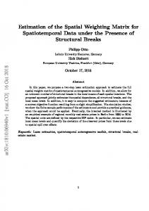
Figure 1: Government Office Regions (GORs) in England and Wales
England and Wales, and advance tentative hypotheses concerning the ‘real’ factors determining spatial diffusion in housing demand.
5.2
The Data
The empirical analysis covers housing markets in England and Wales over the period November 2000 to May 2003. The basic spatial units of analysis are the ten government office regions in England and Wales (Figure 1). Data on regional housing markets for the period have been collected or estimated on a monthly basis. Monthly data on local housing markets at 3-digit postcode level were obtained from Hometrack, an independent property research and database
30
company in the UK16 . The variables included are: • Average number of views; • Average time on the market (TOM); and • Average final to listing price ratios (reciprocal of degree-of-overpricing). Additional regional spatio-temporal data on supply, demand, neighbourhood characteristics and market conditions were collected (see Appendix 1). Data were also collected for other variables useful in interpreting the estimated spatial weights. 5.2.1
Structural Equations
The structural equations of our model of housing markets17 include four relationships in the four endogenous variables — namely, prices, demand, degreeof-overpricing and time on the market. Given the relatively short time-series of our data (monthly from November 2000 to May 2003), and given our focus on understanding spatial diffusion in demand, we present our structural relationships in first differences. This approach renders each of demand, supply, prices, degree-of-overpricing and time on the market stationary across the temporal dimension. In our model, supply and demand both have temporal variation. Demand is endogenously determined but supply is exogenous, and in equilibrium supply (St ) is related to demand (Dt ) as Dt ≡ (1 − ν t ) .St ,
(23)
where ν t denotes the vacancy rate We assume an extended rental adjustment model (Hendershott, 1996), expressed in terms of values rather than rents, relating change in realised value (price) (Vt ) of housing properties to deviations of the vacancy rate from the natural vacancy rate and deviations of the realised value from its 16
The Hometrack data are based on compilation of monthly responses to a questionnaire, from about 3,500 major estate agents in the UK. The data are rather unique in providing information on time on the market and degree-of-overpricing, both of which have important roles in our analysis. We benchmark this information with data from other sources. In particular, we augment the Hometrack data with quarterly information on sales price and number of sales by type of property, for each county and local/ unitary authority, collected from HM Land Registry of England and Wales. 17 For further details on the derivation of these structural equations, see Bhattacharjee and Jensen-Butler (2005).
31
equilibrium level (Vt∗ ). We further assume that the natural value (Vt∗ ) is fixed in the short run (Vt∗ ≡ V ∗ ). Hence, change in realised value (price) is explained by change in occupancy rate (1- vacancy rate), change in natural value, and lagged change in realised value. Since ∆ ln Vt∗ = 0, and ∆ ln(1 − ν t ) ≡ ∆ ln Dt − ∆ ln St , we have: ∆ ln Vt = γ 1 ∆ ln(1 − ν t−1 ) + γ 2 ∆ ln Vt∗ + γ 3 ∆ ln Vt−1 + = γ 1 ∆ ln Dt−1 + γ 3 ∆ ln Vt−1 − γ 4 ∆ ln St−1 + 1t ,
1t
(24)
0 < {γ 1 , γ 3 } < 1, γ 4 = γ 1 . Demand is modelled as a function of realised value, housing market conditions and neighbourhood characteristics. The market conditions include economic activity (Yt ; local and economy-wide income, unemployment, productivity and interest rates) and the neighbourhood characteristics include socio-economic variables (Xt ; quality of education and public services, demographics, etc.). Hence, change in demand is explained by change in local (neighbourhood characteristics), change in price, and change in (local) income or other indicators of local market conditions. ∆ ln Dt = λ1 ∆Xt + λ2 ∆ ln Vt + λ3 ∆ ln Yt +
2t ,
(25)
where λ2 < 0 is the price elasticity and λ3 > 0 may be regarded as the income elasticity. If vacancy rates and supply were perfectly observed, the above three relationships (Equations (23), (24) and (25)) become recursive and the structural relationships can be easily estimated18 . However, quality data on vacancy rates for the residential housing market in the UK are difficult to obtain. Further, even though data on supply of residential property are more readily available, there may be no perceptible changes in supply over time in many non-urban areas. This is because investment in residential property is often highly localized and geographically not very widespread. Hence, supply data do not contain sufficient information to explain temporal variation in the demand-supply balance in regional housing markets. We have therefore drawn on the literature on search, bargaining and price-setting in housing markets (see, for example, Wheaton, 1990; Krainer, 2001; and Anglin et al., 2003) to identify other observed characteristics of the housing markets to identify the wedge between demand and supply. This literature describes the way in which the initial list price (VtL ) is set, the final 18
This is the usual approach taken in the rental office market literature. See, for example, Hendershott et al. (2002) and references therein.
32
(realised) price is determined through repeated search and bargaining by both the seller and the buyer, and the time-on-the-market (T OMt ) that it takes to find an appropriate buyer. The trade-offs between time-on-the-market and setting the initial listing price (equivalently, the degree-of-overpricing, DOPt ) play crucial roles in this price-setting process. A higher list price discourages potential buyers and increases time on the market, while a lower initial list price reduces time on the market but also simultaneously reduces the final price. Broadly following Anglin et al.(2003), we can represent listing price, VtL (= Vt .DOPt ), as a function of demand, market conditions and local neighbourhood characteristics typically included in a hedonic model. It follows that: ∆ ln DOPt = α1 ∆Xt + α2 ∆ ln Yt + α3 .∆ ln Dt − α4 ∆ ln Vt +
4t ,
(26)
α4 = 1. Further, it has been argued that time on the market increases with both the degree-of-overpricing and the vacancy rate, though the relationship with degree-of-overpricing may vary somewhat with the nature of the market (Anglin et al., 2003). Hence, we have: ∆T OMt = β 1 ∆ ln Yt + β 2 ∆ ln DOPt − β 3 ∆ ln Dt + β 4 ∆ ln St +
5t ,
(27)
β4 = β3. The system comprising the above four simultaneous equations (Equations (24), (25), (26) and (27)) is overidentified. Identifiability is not affected if multiple indicators for neighbourhood characteristics and local market conditions are included. The four endogenous variables (∆ ln Vt , ∆ ln Dt , ∆ ln DOPt and ∆T OMt ) are measured in first differences, and tests indicate that each of these variables are stationary over the temporal domain in each of the 10 regions under consideration, as well as in a panel. Hence, we estimate the relationships simultaneously using a 3SLS method, where the spatial autocovariance matrix estimated from the residuals incorporates unrestricted spatial interaction across the different regions. In the first stage of our estimation procedure, we estimate the four structural equations individually for each region, using measures of demand (average number of views per week), realised value (price), degree-of-overpricing, time on the market, neighbourhood characteristics (unfit houses, access to education, and crime detection rates) and indicators of market conditions 33
(claimant counts and average household income). This allows for heterogeneity in the relationships across the regions, both in the sense of intercept heterogeneity (or heterogeneity in spatial fixed effects) and slope heterogeneity, and in the choice of indicators for neighbourhood characteristics and market conditions. In other words, we assume a spatial regime model with a completely general form of heterogeneity across the spatial units. This kind of heterogeneity is desirable in our context, since there is no a priori reason to believe that the functioning of housing markets in different regions will be homogeneous. Under this model, we estimate our structural equations separately for each region using 3SLS, and estimate the spatial autocovariance matrix for the demand equation from the second-stage residuals. It may be mentioned here that the structural disturbance covariance matrix in our case is singular. This is because we use data for 31 months to construct the covariance matrix for 40 structural equations (4 structural equations × 10 regions). Therefore, in the third stage, we estimate our structural equations using the Moore-Penrose generalised inverse of the covariance matrix (Court, 1974). However, the estimated 10 × 10 spatial covariance matrix of the demand equation is still nonsingular. It is well-known that instrumental variables methods can lead to poor results in cross-sectional analysis. Following the literature, we check the Fstatistics of the first stage regressions for each of the endogenous variables in our model, and verify that the instruments in our estimated model are well-specified. The estimates of the structural equations are consistent with a priori expectations19 and qualitatively very similar to the second stage SURE estimates reported in Bhattacharjee and Jensen-Butler (2005). The results are not reported here since we are more interested in analysing the spatial errors from the demand equation; however, we briefly discuss the estimates. We find substantial heterogeneity in the coefficients and in the specification of the relationships across the various regions. For the demand relationship, which is our major focus in this paper, the coefficient of the price variable is negative and significant for most regions, but with substantial slope heterogeneity. Neighbourhood characteristics have an important effect on demand, where share of unfit houses is negatively related to demand in most of the regions, and access to education and crime detection have positive effects. Similarly, market conditions measured by claimant counts and average household income have the expected signs (negative and positive respectively). 19
There is one exception; in the degree-of-overpricing relationship, the estimated coefficient on predicted price is positive but not significant.
34
5.3
Spatial Diffusion of Demand
The spatial autocovariance matrix of demand is estimated non-parametrically, (i.e., without specifying any explicit spatial process or functional form for the distance decay) from the second-stage residuals of the demand equation. Separate equations are estimated for each region, and we allow unexplained variation in demand to be contemporaneously correlated across the regions. This approach is consistent with the spatial regime model allowing heterogeneity in the demand relationship across regions. Further, the approach allows for completely unrestricted kinds of spatial autocorrelation in the regressuion errors. This estimated spatial autocovariance matrix is used to d (Equation 16). estimate the implied matrix of spatial weights, ρW Table 4: Estimated Error Covariance and Correlation Matrices20 A. Errors, Spatial Autocovariance Matrix E E EM L NE NW SE SW W WM YH
E EM L NE NW SE SW W WM YH
0.011 0.011 0.005 0.017 0.003 0.008 0.003 0.019 0.005 0.022
EM
L
0.018 0.008 0.007 0.027 0.015 0.004 0.003 0.009 0.006 0.003 0.002 0.029 0.016 0.008 0.006 0.031 0.017 B. Errors,
E
EM
1 0.764 0.589 0.605 0.191 0.813 0.352 0.495 0.526 0.614
1 0.688 0.741 0.241 0.717 0.217 0.607 0.605 0.707
L
NE
NW
SE
SW
W
WM
YH
0.073 0.003 0.015 0.015 0.001 0.008 −0.000 0.007 0.002 0.008 0.082 −0.009 0.019 −0.008 0.128 0.014 0.004 0.005 0.004 0.012 0.009 0.080 −0.004 0.019 −0.004 0.104 0.013 0.109 Spatial Autocorrelation Matrix NE
NW
SE
SW
W
WM
1 0.640 1 0.260 0.081 1 0.750 0.634 0.092 1 0.314 −0.007 0.635 0.284 1 0.524 0.845 −0.205 0.581 −0.241 1 0.672 0.522 0.317 0.593 0.457 0.342 1 0.608 0.890 −0.100 0.631 −0.117 0.877 0.415
20
E: East of England; EM : East Midlands; L: Greater London; N E: North East; N W : North West; SE: South East; SW : South West; W : Wales; W M : West Midlands; Y H: Yorks & Humberside.
35
YH
1
The spatial autocovariance matrix across the 10 regions (Table 4 A) and the corresponding spatial autocorrelation matrix (Table 4 B) show some interesting spatial characteristics. Housing demand in Greater London is strongly correlated with the South East, and also with West Midlands. The highest spatial correlations are observed for Wales and Yorkshire and Humberside, North East and Yorkshire and Humberside, North East and Wales and East and the South East. These patterns indicate that spatial patterns in demand are not necessarily related to simple notions of contiguity and geographical distance. For example, demand diffusion in London is not strongly related to the East of England, which is contrary to common perception. Similarly, the strong correlation between London and West Midlands, between Wales and North East and between Wales and Yorkshire and Humberside are somewhat difficult to justify based on geographical distance notions. It is possible that the nature of diffusion is related to the structure of the urban hierarchy, or peripherality, or perhaps even topologically in terms of networks. In order to understand the nature of spatial diffusion in terms of spad (Equation 16) to estimate the spatial tial weights, we use our estimator ρW weights matrix implied by the spatial autocovariance matrix reported in Table 4, under the assumption of a spatial error model with autoregressive errors (Equation 1). These estimates, reported in the top panel of Table 5 (Table 5A), measure the spatial contribution of demand in other regions to the determination of housing demand in each individual region. Put differently, the elements in a row corresponding to the index region represent, within the context of the estimated spatial autoregressive model, the contributions of idiosyncratic excess demand from other regions to excess demand in the index region. The corresponding estimated row-standardised spatial weights matrix is reported in the lower panel of Table 5 (Table 5B). Bootstrap 95 percent confidence intervals for each element of the spatial weights matrix, and the estimates of region-specific standard deviations of the spatial errors are also reported in Table 5A. Below we describe the bootstrap procedure and the construction of confidence intervals. Based on the 3SLS procedure described in the previous subsection, we propose the following bootstrap procedure: 1. Estimate the structural equations using the 3SLS procedure for singular covariance matrix (Court, 1974), and compute a set of 31 residual vectors for the four endogenous variables, one set for each time period. bt , t = 1, . . . , 31, where ¡ Let us denote these residual ¢ vectors u b(V )t , u b(D)t , u b(DOP )t , u b(T OM)t and the estimates of the parameu bt = u ters of the structural equations α b. 36
2. Draw a bootstrap sample u b∗t , t = 1, . . . , 31 from the empirical distribution of the residuals u bt .
3. For each bootstrap trial, take the exogenous and predetermined variables and the residuals as given and obtain estimates for the endogenous b ,b u∗t ), variables in the sequence ∆ ln Vbt (∆ ln Dt−1 , ∆ ln Vt−1 , ∆ ln St−1 ; α b t, b t (∆Xt , ∆ ln Vbt , ∆ ln Yt ; α \t (∆Xt , ∆ ln Yt , ∆ ln D b ,b u∗t ), ∆ ln DOP ∆ ln D b t , ∆ ln St ; α \t , ∆ ln D b ,b u∗t ) and ∆T\ OM t (∆ ln Yt , ∆ ln DOP b ,b u∗t ) for ∆ ln Vbt ; α t = 1, . . . , 31.
4. Using these predicted values for the endogenous variables, run the first and second stage of the 3SLS procedure. Using the reduced form residuals, compute the spatial covariance matrix and its eigen-decomposition. Use the eigenvalues and corresponding eigenvectors compute the estimate of the spatial weights matrix. 5. Repeat steps 2—4 for each bootstrap trial.
Using this bootstrap procedure, we generate 200 bootstrap replications of the estimated spatial weights matrix. We also compute 31 jackknife replications of the spatial weights matrix by omitting one time period each time. For each element of the spatial weights matrix, we compute 95 percent confidence intervals using the nonparametric BCα accelerated bootstrap confidence intervals (DiCiccio and Efron, 1996). The bias correction term in the confidence interval is estimated nonparametrically while the acceleration parameter is estimated using the jackknife. The bootstrap confidence limits are used to identify statistically significant spatial weights in Table 5A. Several elements in the estimated symmetric spatial weights matrix (Table 5 A) are significantly different from zero, either positive or negative. Similarly, several contributions in the row-standardized matrix (Table 5 B) are numerically large (indicated in bold), suggesting a significant contribution from some regions to demand in the index region. For example, in relation to housing demand in Greater London (L, row 3 in Table 5B), 34 percent of the spatial diffusion originates from West Midlands, 30 percent from the East of England, and another 20 percent from the South East; while the contribution from Yorkshire and Humberside is 24 percent, that from the contiguous region North East is significantly negative at minus 25 percent. The corresponding contributions in the spatial weights matrix (Table 5 A) are significant at at least the 10 percent level of significance. Below, we examine the pattern of these significant weights in order to understand the process of spatial diffusion lying behind the observed demand for housing in 37
the different regions. Our findings are consistent with the view that the nature of spatial diffusion in regional housing markets is more complicated than what can be modeled using a single and simple notion of distance. In particular, we find several explanations, singly or in combination, for the pattern of observed spatial diffusion; these include geographic contiguity or distance, inter-regional economic interactions, and social interactions and segregation. First, contiguity or distance explains a number of the significant positive spatial weights. These include: spatial weights between Greater London, South East and the East of England; North East and Yorkshire and Humberside; and spatial weights of West Midlands with the neighbouring regions East Midlands and the South West. Tentative explanations can be offered. Greater London, the South East and East can be regarded as substitutes in the choice of housing location. Hence, idiosyncratic shocks to housing demand in one of these regions can also affect demand in the other two regions. It is, however, interesting to note that the demand in the North West is negatively related to that in Wales, and not significantly related to housing demand in Yorkshire and Humberside; similarly the spatial weight between Wales and neighbouring regions South West and North West are significantly negative. This suggests that the regional markets may be segmented in social or ethnic terms, implying that while the North West may be attractive for certain social groups, these groups may be less attracted to housing market in the neighbouring regions21 . On the other hand, many other significant spatial weights appear to be driven by reasons other than geographic distance or contiguity. A test for the first-order contiguity spatial weights matrix using the proposed test statistic (Equation 22) also rejects the specified driver of spatial diffusion in demand at the 1 per cent level of significance. This evidence also supports the view that there is more to the nature of spatial dependence than what can be explained by simple geographic distances. Second, a few of the strong positive spatial interactions operate along major inter-region transport links. Significant positive spatial weights of Yorkshire and Humberside with Greater London and the South East; between the North East and West Midlands; and similarly between the North West and the South West appear to be related to transportation infrastructure (railways and motorways). This evidence is in line with recent evidence on the effect of commuting time and choice on housing demand (Gibbons and Machin, 2005).
21
Meen and Meen (2003) point to the importance of social interactions and segregation in understanding housing markets.
38
E E EM L NE NW SE SW W
Table 5: Estimated Spatial Weights Matrix22 d A. Symmetric Spatial Weights Matrix, ρW
0 0.17
(-.13,.33) ∗∗
0.30
0.02
−0.26∗∗
(-.29,.20)
−0.16
(-.08,.53)
(-.45,.16) ∗∗
0.46
(.29,.64) ∗∗
0.34
(.19,.52)
−0.03
(-.44,-.03)
0.00
(-.28,.18)
.039∗∗
(.02,.06)
E E EM L NE NW SE SW W WM YH
0
(-.02,.47)
WM −0.25
σ ck
−0.02
(-.23,.17)
0.22
0 0.23 0.30 0.19 −0.42 0.34 0.54 −0.07 −0.33 0.00
L
NE
NW
SE
SW
W
WM
YH
0
(.16,.62) +
(-.27,.27) ∗∗
YH
EM
0.19 0.05
0.18
(-.11,.27) +
0.20
(-.19,.19)
(-.04,.45)
−0.05
(-.29,.22)
(-.31,.21)
0.05
(-.22,.27) +
0.15
(-.04,.46)
0.16
(-.06,.48)
.068∗∗
(.05,.08)
0
(-.42,-.22)
−0.03 0.05
(-.16,.24) ∗∗
0.35
(.08,.56) ∗∗
0.24
(.10,.37)
.040∗∗
(.03,.05)
0.22+
(-.05,.55) ∗
−0.26
(-.62,.44)
0.05
(-.28,.20) ∗∗
0.41
(.22,.66) ∗∗
0.47
0 0.09
(-.13,.53) ∗
0.39
0.24
−0.19+
(-.50,.12) ∗
(-.16,.58) ∗∗
−0.08
(.18,.46)
−0.20
−0.22
(-.08,.51)
(-.31,.16) ∗∗
.088∗∗
0
(-.43,.11)
(-.53,-.04)
(.05,.13)
−0.04
(.02,.78) +
(.26,.79) +
0.32
0
.077
(.05,.11)
0.36
(.18,.70) ∗
0.28
.034∗∗
(.02,.05)
(-.40,-.08) ∗∗
0.21
(.05,.43)
−0.05
(-.30,.30) ∗∗
.044
(.03,.06)
0 −0.20
(-.55,.12) ∗∗
0.32
(.12,.71)
.122∗∗
(.03,.21) (RS)
c B. Row-Standardised Spatial Weights Matrix, W EM
L
0.16 0 −0.02 0.02 0.49 0.04 −0.07 0.12 0.20 0.16
0.28 −0.03 0 −0.22 0.45 0.14 −0.05 0.11 0.46 0.22
NE
NW
SE
SW
W
0 −0.11∗
(-.25,-.03) ∗∗
.041
0 .114∗∗
(.01,.07)
(.05,.20)
WM
YH
23
0.21 −0.15 0.43 0.31 −0.02 −0.23 0.01 0.03 0.26 0.07 −0.06 0.08 0.21 0.23 −0.25 0.17 0.20 −0.03 0.05 0.34 0.24 0 0.18 −0.23 0.04 0.35 0.39 0.27 0.55 0 0.23 0.98 −0.51 −0.57 −0.20 −0.19 0.06 0 −0.03 0.18 0.26 0.20 0.09 0.62 −0.07 0 −0.30 0.33 −0.07 0.94 −0.46 0.54 −0.44 0 −0.47 0.72 0.61 −0.30 0.47 0.27 −0.26 0 −0.13 0.30 −0.08 0.26 −0.05 0.30 −0.10 0
22
Abbreviations for the regions are as in Table 4. , , : Significant at 10 per cent, 5 per cent and 1 per cent level respectively.
+ ∗ ∗∗ 23
Figures in bold in the estimated row-standardised spatial weights matrix denote the numerically “large” spatial weights in each row (positive or negative), without attaching any probabilistic interpretation to these figures.
39
Third, the housing markets in some more peripheral regions, like Wales, North East and Yorkshire and Humberside, appear to be related reciprocally. Spatial weights between Wales on the one hand and Yorkshire and Humberside and the North East on the other are positive and highly significant; further, the contiguous regions Yorkshire and Humberside and North East also have significantly high spatial weights. One possible interpretation is that an external shock affects the periphery as a whole differently, and in some senses uniformly, compared to other regions. Fourth, the spatial weights between West Midlands (which is dominated by Birmingham) and Greater London and the South East are positive and significant at the 1 per cent level. This evidence suggests that shocks to local demand in West Midlands may similarly affect housing demand in Greater London. One could also propose the hypothesis that social interactions in substantial market segments in either region (for example, segments constituted by different ethnic groups) may play a crucial role. This is also in line with recent evidence on immigrant networks and inter-region trade (Herander and Saavedra, 2005). The significant spatial weight between the South West and the North West (dominated by Manchester) could also be driven by similar reasons. The strong spatial relationship between the North West and the South West is particularly important because the North West has low and insignificant spatial weights with most of the other regions; an explanation could have implications for understanding the nature of ripple effects in the UK housing markets. The significant spatial weight between the East of England and the South West may also be explained similarly. Finally, Table 5 A indicates some negative spatial interactions in the spatial weights for North East with Greater London and the South East, and for Wales with the North West and the South West. These negative spatial weights would suggest one of two possibilities. First, the housing markets in the South West, Wales and North West could be alternatives with respect to housing for retirement. Second, the negative spatial weights between the North East and regions in the south may be related to the “ripple effects” phenomenon, whereby sharp changes in housing markets in the South East and London slowly spread over time to other parts of the country. This could imply that different regions may be on different housing market cycles, which are possibly asynchronous with one another. In summary, the application identifies significant and interpretable spatial relationships in demand between government office regions in England and Wales, based on an estimate of the symmetric spatial weights matrix. We find that while contiguity and geographic distance provide some understanding of the strength of inter-region interactions, other factors such as socio-cultural 40
distances and transport infrastructure may also drive the spatial diffusion in housing demand. This is in addition to the importance of neighbourhood characteristics such as educational facilities and crime that has been noted in the literature (Cheshire and Sheppard, 2004; Gibbons, 2004). A more complete analysis of these effects would involve constructing spatial weights matrices reflecting the drivers suggested by the current work, and then to formally examine the explanatory power of corresponding spatial weights. Recent methodological advances in Conley (1999), Pinkse et al. (2002) and Kelejian and Prucha (2004) could provide important tools for such extension of the current analysis.
6
Conclusion
The paper proposes a methodology for estimation of a symmtric spatial weights matrix, based on consistent estimators for the spatial autocovariances. The methodology has the important advantage that it does not assume the availability of any distance measures or spatial weights, nor any a priori assumption about the nature of spatial diffusion. This flexible (nonparametric) approach to studying spatial diffusion represents a departure from the literature. We discuss various features of the estimator including its large sample properties, outline a bootstrap procedure for computing standard errors, and propose a test for a specified driver of spatial diffusion. Results of a Monte Carlo simulation study demonstrate the superior small-sample performance of the proposed estimators. The proposed methodology is used to study spatial diffusion in housing demand between government office regions in England and Wales. The spatial weights matrix is estimated and tentative explanations for significant spatial weights are advanced. The structural economic model provides a good description of housing markets in different regions of England and Wales, and the estimates suggest significant heterogeneity in the operation of regional housing markets. The nature and strength of diffusion in the different regions appears to be driven by a combination of factors including contiguity or distance, peripherality, as well as social, ethnic, and national composition representing cultural distance, none of which is a priori obvious. Besides, some other regions have negative spatial weights which can be explained by substitution effects or by “ripple effects”. Thus, our approach provides substantial information about the nature of spatial diffusion, is useful both in explaining how regional housing markets function, and in the evaluation of region-specific housing and related policies. 41
The work in this paper suggests several extensions and paths of model development. These include: further analysis using spatial weights matrices which incorporate the drivers of spatial diffusion identified in this paper; analysis at a lower level of spatial disaggregation; and extending our modeling approach in relation to spatial diffusion to include temporal aspects thereby improving understanding of features such as ripple effects. Extension of the methodology to other models of spatial interaction will enhance the usefulness of the methodology. Similar analyses can uncover dimensions of spatial interaction in other applications, such as the study of convergence across regions and more generally in applied microeconomic studies of cross-sectional dependence.
References [1] Anglin, P.M, Rutherford, R. and Springer, T.M. (2003). The trade-off between selling price of residential properties and time-on-the-market: The impact of price setting. Journal of Real Estate Finance and Economics 26, 95—111. [2] Anselin, L. (1988). Spatial Econometrics: Methods and Models. Kluwer Academic Publishers: Dordrecht, The Netherlands. [3] Anselin, L. (1999). Spatial econometrics. In Baltagi, B.H. (Ed.), A Companion to Theoretical Econometrics. Oxford: Basil Blackwell, 310—330. [4] Anselin, L. (2001). Rao’s score tests in spatial econometrics. Journal of Statistical Planning and Inference 97, 113—139. [5] Anselin, L. (2002). Under the hood: Issues in the specification and interpretation of spatial regression models. Agricultural Economics 27, 247—267. [6] Aten, B. and Heston, A. (2005). Regional output differences in international perspective. In Kanbur, R. and Venables, A.J. (Eds.) Spatial Inequality and Development. UNU-Wider Studies in Development Economics, Oxford University Press: New York. [7] Baltagi, B., Song, S.H. and Koh, W. (2003). Testing panel data regression models with spatial error correlation. Journal of Econometrics 117, 123—150. [8] Barker, K. (2003). Review of Housing Supply. Interim Report, HM Treasury: London. 42
[9] Barro, R.J. and Sala-i-Martin, X. (1992). Convergence. Journal of Political Economy 100, 223—251. [10] Bell, K.P. and Bockstael, N.E. Applying the generalized-moments estimation approach to spatial problems involving microlevel data. The Review of Economics and Statistics 82, 72—82. [11] Beran, R. and Srivastava, M.S. (1985). Bootstrap tests and confidence regions for functions of a covariance matrix. The Annals of Statistics, 13, 95—115. [12] Bhattacharjee, A. and Jensen-Butler, C. (2005). A model of regional housing markets in England and Wales. CRIEFF Discussion Paper No. 0508, Centre for Research into Industry, Enterprise, Finance and the Firm, University of St. Andrews. [13] Brown, B.W. and Mariano, R.S. (1984). Residual-based procedures for prediction and estimation in a nonlinear simultaneous system. Econometrica 52, 321—343. [14] Cheshire, P. and Sheppard, S. (2004). Capitalising the value of free schools: The impact of supply constraints and uncertainty. Economic Journal 114, F397—F424. [15] Conley, T.G. (1999). GMM estimation with cross sectional dependence. Journal of Econometrics 92, 1—45. [16] Court, R.H. (1974). Three stage least squares and some extensions where the structural disturbance covariance matrix may be singular. Econometrica 42(3), 547—558. [17] DiCiccio, T.J. and Efron, B. (1996). Bootstrap confidence intervals. (with discussion and a rejoinder). Statistical Science 11(3), 189—228. [18] Fair, R.C. (2003). Bootstrapping macroeconometric models. Studies in Nonlinear Dynamics and Econometrics 7, 4, Article 1. [19] Fik, T.J., Ling, D.C. and Mulligan, G.F. (2003). Modeling spatial variation in housing prices: A variable interaction approach. Real Estate Economics 31, 623—646. [20] Fingleton, B. (2003). Externalities, economic geography and spatial econometrics: conceptual and modeling developments. International Regional Science Review 26, 197—207. 43
[21] Freedman, D. (1984). On bootstrapping two-stage least squares estimates in stationary linear models. The Annals of Statistics 12, 827—842. [22] Freedman, D. and Peters, S.C. (1984). Bootstrapping a regression equation: Some empirical results. Journal of the American Statistical Association 79, 97—106. [23] Giacomini, R. and Granger, C.W.J. (2004). Aggregation of space-time processes. Journal of Econometrics 118, 7 — 26. [24] Gibbons, S. (2004). The costs of urban property crime. Economic Journal 114, F441—F463. [25] Gibbons, S and Machin, S. (2005). Valuing rail access using transport innovations. Journal of Urban Economics 57, 148—169. [26] Haurin, D.R. and Brasington, D. (1996). School quality and real house prices: intra- and interjurisdictional effects. Journal of Housing Economics 5, 351—368. [27] Hendershott, P. (1996). Rental adjustment and valuation in overbuilt markets: Evidence from the Sydney office market. Journal of Urban Economics 39, 51—67. [28] Hendershott, P., MacGregor, B. and White, M. (2002). Explaining real commercial rents using an error correction model with panel data. Journal of Real Estate Finance and Economics 24, 59—87. [29] Herander, M.G. and Saavedra, L.A. (2005). Exports and the structure of immigrant-based networks: the role of geographic proximity. Review of Economics and Statistics 87, 323—335. [30] Horowitz, J.L. (2001). The bootstrap. In Heckman, J.J. and Leamer, E.E. (Eds.) Handbook of Econometrics, Vol. 5, Elsevier Science B.V., Chapter 52, 3159—3228. [31] Jennrich, R.I. (2001). A simple general procedure for orthogonal rotation. Psychometrika 66, 289—306. [32] Jennrich, R.I. (2004). Derivative free gradient projection algorithms for rotation. Psychometrika 69, 475—480. [33] Kelejian, H.H. and Prucha, I.R. (1999). A generalized moments estimator for the autoregressive parameter in a spatial model. International Economic Review 40, 509—533. 44
[34] Kelejian, H.H. and Prucha, I.R. (2004). Estimation of systems of spatially interrelated cross sectional equations. Journal_ of_ Econometrics 118, 27—50. [35] Krainer, J. (2001). A theory of liquidity in residential real estate markets. Journal of Urban Economics 49, 32—53. [36] Lacombe, D.J. (2004). Does econometric methodology matter? An analysis of public policy using spatial econometric techniques. Geographical Analysis 36, 105—118. [37] Ledoit, O. and Wolf, M. (2002). Some hypothesis tests for the covariance matrix when the dimension is large compared to the sample size. The Annals of Statistics 30, 1081—1102. [38] Mardia, K.V. and Marshall, R.J. (1984). Maximum likelihood estimation of models for residual covariance in spatial regression. Biometrika 71, 135—146. [39] Meen, G. (1996). Spatial aggregation, spatial dependence and predictability in the UK housing market. Housing Studies 11, 345—372. [40] Meen, G. (1999). Regional house prices and the ripple effect: A new interpretation. Housing Studies 14, 733—753. [41] Meen, G. (2001). Modelling Spatial Housing Markets: Theory, Analysis and Policy. Kluwer Academic Publishers: Boston. [42] Meen, G. (2003). Regional housing supply elasticities in England. Report prepared for the Barker Review of Housing Supply. Centre for Spatial and Real Estate Economics, University of Reading, October 2003. [43] Meen, D. and Meen, G. (2003). Social Behaviour as a Basis for Modelling the Urban Housing Market: A Review. Urban Studies 40, 917—935. [44] Muirhead, R.J. (1982). Aspects of Multivariate Statistical Theory. Wiley: New York. [45] Ord, J.K. (1975). Estimation methods for models of spatial interaction. Journal of the American Statistical Association 70, 120-126. [46] Pinkse, J., Slade, M.E. and Brett, C. (2002). Spatial price competition: a semiparametric approach. Econometrica 70, 1111—1155.
45
[47] Rey, S.J. and Montouri, B.D. (1999). US regional income convergence: a spatial econometric perspective. Regional Studies 33, 143—156. [48] Rilstone, P. and Veall, M. (1996). Using bootstrapped confidence intervals for improved inferences with seemingly unrelated regression equations. Econometric Theory 12, 569—580. [49] Rosenthal, S. (1999). Residential buildings and the cost of construction: New evidence from the housing market. Review of Economics and Statistics 81, 288—302. [50] Staiger, D. and Stock, J. (1997). Instrumental variables regression with weak instruments. Econometrica 65, 557—586. [51] Wheaton, W.C. (1990). Vacancy, search and prices in a housing market matching model. Journal of Political Economy 98, 1270—1292. Appendix 1: Sources of spatio-temporal data Other than Hometrack, sources for regional spatio-temporal data were: • Supply: Housing stock (Source: Office of the Deputy Prime Minister (ODPM) and the Office of National Statistics (ONS); • Demand: Proportion of Local Authority and RSL dwellings having low demand (Source: ODPM); Property transactions (Source: HM Land Registry and Inland Revenue); Supply minus vacant housing (Source: ODPM); Average number of views per week (Source: Hometrack); • Neighbourhood characteristics: Percentage of unfit houses (Source: ODPM); Crime rates (Source: ODPM); Crime detection rates (Source: Home Office); Percentage of university acceptances to applications (Source: Universities and Colleges Admissions Service (UCAS)); Percentage of population of 16-24 year olds attending university (Source: UCAS); Best value performance indicators (Source: ODPM); and • Market conditions: Average weekly household income (Source: ONS); unemployment rate (Source: Labour Force Survey (LFS)); Proportion of population claiming income support (Source: ONS).
46