2212
JOURNAL OF THE ATMOSPHERIC SCIENCES
VOLUME 67
Evaluating Boundary Layer–Based Mass Flux Closures Using Cloud-Resolving Model Simulations of Deep Convection JENNIFER K. FLETCHER AND CHRISTOPHER S. BRETHERTON University of Washington, Seattle, Washington (Manuscript received 21 September 2009, in final form 24 February 2010) ABSTRACT High-resolution three-dimensional cloud resolving model simulations of deep cumulus convection under a wide range of large-scale forcings are used to evaluate a mass flux closure based on boundary layer convective inhibition (CIN) that has previously been applied in parameterizations of shallow cumulus convection. With minor modifications, it is also found to perform well for deep oceanic and continental cumulus convection, and it matches simulated cloud-base mass flux much better than a closure based only on the boundary layer convective velocity scale. CIN closure maintains an important feedback among cumulus base mass flux, compensating subsidence, and CIN that keeps the boundary layer top close to cloud base. For deep convection, the proposed CIN closure requires prediction of a boundary layer mean turbulent kinetic energy (TKE) and a horizontal moisture variance, both of which are strongly correlated with precipitation. For our cases, CIN closure predicts cloud-base mass flux in deep convective environments as well as the best possible bulk entraining CAPE closure, but unlike the latter, CIN closure also works well for shallow cumulus convection without retuning of parameters.
1. Introduction Large-scale general circulation models (GCMs) employ a diverse range of parameterizations for shallow (i.e., most weakly precipitating) and deep (i.e., heavily precipitating) cumulus (Cu) convection. Most cumulus parameterizations use a mass flux approach, which predicts the vertical structure and mass flux of cumulus up- and downdrafts in the parameterization. Mass flux schemes are popular because they can provide an internally consistent treatment of cloud turbulent mixing, tracer transport, and, if coupled to a parameterization of updraft velocity, cumulus microphysics. In these schemes, the cumulus-base (Cu-base) updraft mass flux per unit horizontal area in each grid cell must be specified using a mass flux closure that relates upward mass flux in the cumulus cloud base to model-predicted variables. A plume or plume ensemble model then predicts the vertical structure of mass flux and thermodynamic variables such as updraft temperature, liquid water content, and precipitation flux. There is still no consensus on the proper approach to mass flux closure. Historically speaking, the first closure
Corresponding author address: Jennifer Fletcher, University of Washington, 408 ATG Bldg., Seattle, WA 98195–1640. E-mail:
[email protected] DOI: 10.1175/2010JAS3328.1 Ó 2010 American Meteorological Society
type was moisture convergence, proposed by Kuo (1974) and extended by Anthes (1977) and Molinari (1982). Under such closure, convection develops to balance columnintegrated moisture convergence. Such a balance is observed over the tropical oceans on long time scales. However, on the shorter time scales over which convection evolves, moisture convergence closure is unphysical. This is because convection is fundamentally a buoyancydriven process and hence must develop as a response to local thermodynamic profiles rather than to large-scale fields. Furthermore, moisture convergence closure requires ad hoc assumptions about the storage term in the moisture budget. For these reasons, moisture convergence closure has gradually lost popularity. Many current deep convective parameterizations use a convective quasi-equilibrium closure assumption that adjusts the cloud-base mass flux to regulate convective available potential energy (CAPE)— or an entraining variant of it—in the face of destabilization by nonconvective processes. Arakawa and Schubert (1974), Bechtold et al. (2001), Zhang and McFarlane (1995), and Fritsch and Chappell (1980) all used closures based solely on CAPE. However, observational and modeling studies (e.g., Mapes and Houze 1992; Neggers et al. 2004; Grabowski et al. 2006; Sobel et al. 2004; Kuang and Bretherton 2006, hereafter KB) have found CAPE to be poorly correlated
JULY 2010
FLETCHER AND BRETHERTON
with rainfall or cloud-base mass flux. Estimates of entraining CAPE (ECAPE)—the vertically integrated positive buoyancy of cumulus updrafts, also called the cloud work function by Arakawa and Schubert (1974)— are observed to be better correlated with tropical oceanic deep convective rainfall (e.g., Brown and Zhang 1997). The relaxed Arakawa–Schubert scheme (Moorthi and Suarez 1992) separately regulates the entraining CAPE of multiple cumulus updrafts with a spectrum of assumed entrainment rates. Entraining CAPE mass flux closure schemes tend to involve many empirically tuned parameters. In this paper, we will focus on a third mass flux closure type, which we call boundary layer (BL)-based closure. In BL-based closure, the cumulus-base mass flux is determined so as to maintain dynamical compatibility between the subcloud turbulent boundary layer and the base of the cumulus cloud layer. Although BL-based closure is not yet widely used in deep cumulus parameterizations, previous researchers have proposed different types of BL-based closure in a variety of contexts. For instance, Raymond (1995), in a study of the Tropical Ocean and Global Atmosphere Coupled Ocean–Atmosphere Response Experiment (TOGA COARE) west Pacific warm pool intensive observing period, proposed that cloud-base mass flux is regulated by boundary layer quasi-equilibrium (BLQ), in which the subcloud boundary layer equivalent potential temperature ue is maintained near a constant convective threshold value through a balance between the increase of conditional instability by surface fluxes and its destruction by low-ue convective downdrafts. Such equilibrium may occur in tropical oceanic deep convective regimes. However, diurnal and synoptic-scale variations of BL ue in convective regions over land are too large to be consistent with BLQ. Furthermore, BLQ cannot apply to shallow cumulus convection, in which significant downdrafts are not present and the subcloud layer is instead ventilated by dry entrainment. Another BL-based mass flux closure was suggested by Mapes (2000), who hypothesized that cloud-base mass flux is controlled by the ratio of the kinetic energy of turbulent updrafts in the subcloud boundary layer to the potential energy barrier that they must overcome. This potential energy barrier is the convective inhibition (CIN), the vertically integrated negative buoyancy of the updrafts. In a highly idealized model of cumulus convection, he proposed a cloud-base mass flux closure of the form mcb 5 W exp( kCIN/W 2 ),
(1)
where mcb is the cloud-base volume flux, W is a measure of the vertical velocity scale of typical boundary layer
2213
eddies, and k is a constant. We will refer to this as CIN closure. A nice feature of this closure is that it requires no separate convective trigger; if CIN gets large, the mass flux turns off. Grant and Brown (1999) found that the ratio of cloudbase mass flux per unit density to the BL convective velocity scale w* 5 (B0h)1/3, where B0 is the surface buoyancy flux and h is the boundary layer depth, was close to 0.03 in several large-eddy simulations of continuously forced shallow convection. This demonstrates the tight connection between boundary layer turbulence and cloud-base mass flux in this situation. This is compatible with CIN closure with W } w* if CIN adjusts to be proportional to W2, in which case exp(2kCIN/W2) is constant. We will call this the Grant closure; for use in a cumulus parameterization it must be supplemented by a trigger function. Neggers et al. (2009) developed a coupled boundary layer and shallow cumulus parameterization that uses a closure that has features in common with CIN closure. In their closure, a weakly entraining test updraft originating in the surface layer is used to determine whether any cumulus clouds are possible and, if so, to diagnose a cumulus layer depth. The cumulus-base updraft fractional area (and hence cumulus-base mass flux) is proportional to the cumulus layer depth up to a maximum proportional to w*/N, where N is an estimated dry static stability at the cloud base h. In this closure, the test parcel cumulus layer depth is used in place of a subcloud layer CIN, N is used in place of a transition layer CIN, and updraft velocity is scaled with w*. In deep convection, the effects of cold pools can often swamp those of surface fluxes on boundary layer properties, as we will show. The CIN closure defined in Eq. (1) can maintain reasonable cumulus-base mass flux even in this case, while that of Neggers et al. (2009) may not. Many GCMs use separate parameterizations for shallow and deep convection. While mass flux-based deep cumulus parameterizations tend to use CAPE and moisture convergence closures, some shallow cumulus parameterizations have used BL-based closures. For instance, Bretherton et al. (2004, hereafter B04) used a shallow cumulus parameterization incorporating CIN closure, basing W on a parameterized boundary layer mean turbulent kinetic energy (TKE), in simulations of the subtropical marine stratocumulus to trade cumulus transition. KB built further evidence for the utility of CIN closure in a simulation of an idealized shallow-to-deep cumulus transition using a cloud-resolving model (CRM). Their results suggested that this closure may be applicable to deep convection as well as to shallow convection. However, KB’s simulation never produced area-mean precipitation rates exceeding 3 mm day21.
2214
JOURNAL OF THE ATMOSPHERIC SCIENCES
In this paper, we follow KB in employing CRM simulations to test cloud-base mass flux closure assumptions. We extend their analysis to include realistic cases of heavily precipitating oceanic and continental deep convection. Specifically, we test a CIN closure of the form mcb 5 c1W exp( c2 CIN/TKE),
(2)
where c1 and c2 are constants to be determined from studies such as this one and W may depend on w*, TKE, or both. The goal is to find a closure that reasonably predicts the mass flux in deep continental and oceanic convection as well as shallow cumulus convection without changes to any parameters. We also test the assumptions behind CAPE closure and the Grant closure. Section 2 briefly describes our CRM and our simulations. Section 3 explains our analysis methods for evaluating each closure, and section 4 presents our results, which favor a form of CIN closure. In section 4 we also discuss how CIN closure and a cloud model act together to maintain convective quasi-equilibrium in a layer of cumulus convection. Section 5 summarizes our conclusions and some remaining challenges.
2. Simulations We use several versions of the System for Atmospheric Modeling (SAM) CRM (Khairoutdinov and Randall 2003) for all our studies. SAM uses the anelastic equations, bulk microphysics, and periodic lateral boundary conditions with a rigid lid upper boundary condition, applying Newtonian damping in the upper model levels. The model’s prognostic thermodynamic variables are total nonprecipitating water content (diagnostically separated into vapor and cloud water/ice using temperature and pressure), total precipitating water (rain, snow, and graupel), and liquid/ice static energy. We use SAM to simulate three well-observed case studies covering a range of environments in which cumulus convection occurs. All have been the subject of prior CRM studies. The cases used were taken from the Atmospheric Radiation Measurement (ARM) Southern Great Plains campaign, the Kwajalein Experiment (KWAJEX), and the Barbados Oceanographic and Meteorological Experiment (BOMEX). Simulations of ARM and BOMEX with earlier versions of SAM are discussed in detail in Khairoutdinov and Randall (2003) and Siebesma et al. (2003), respectively, while our KWAJEX simulation is the same as that discussed in Blossey et al. (2007). The ARM case features summertime midlatitude continental convection and includes suppressed and shallow convective conditions as well as episodic deep convection. Our simulation uses a subperiod of the original ARM case study,
VOLUME 67
from 18 June to 3 July 1997 (Julian days 170–185). The KWAJEX case features continuously forced tropical marine deep convection over the west Pacific warm pool, spanning 23 July–4 September 1999 (Julian days 204–257). The BOMEX case is a 6-h simulation of shallow trade cumuli using steady forcing derived from observations during 22–23 June 1969. Our ARM simulation uses version 6.7 of SAM. It has a 192 3 192 km2 domain, with 1-km grid spacing in the horizontal, 96 vertical grid levels, and a vertical grid spacing varying from 50 to 100 m at the lowest levels to 250 m in the free troposphere, with larger spacing above the tropopause. Our KWAJEX simulation uses version 6.3 of SAM, a 256 3 256 km2 grid, and 1-km grid spacing. It has 64 vertical grid levels with a vertical grid spacing ranging about 100 m at lower levels, 400 m in the free troposphere, and larger spacing above. Our BOMEX simulation uses version 6.6 of SAM, a 192 3 192 km2 3 96 grid, and 40-m grid spacing in both the horizontal and vertical. For each simulation, SAM saves three-dimensional volume snapshots of temperature, horizontal and vertical winds, and water content. These snapshots are archived every hour for ARM, every 6 h for KWAJEX, and every 20 min for BOMEX. The ARM and KWAJEX archival times are comparable to the time scales on which deep convection evolves over land and tropical oceans, as largescale forcings over a continental environment change much more rapidly than they do over a tropical ocean. The BOMEX snapshots can be regarded as statistically independent samples of a quasi-steady shallow cumulus cloud field. Time and horizontal averages of numerous other quantities, including rainfall and surface fluxes, are saved every hour in ARM and KWAJEX and every 10 min in BOMEX. To minimize spinup transients, we do not analyze the first day of the ARM and KWAJEX simulations or the first 3 h of the BOMEX simulations.
3. Methods We define Cu updrafts as saturated updrafts with vertical velocity w . 0.5 m s21. This definition accounts for most of the saturated updraft mass flux while filtering out gravity wave–induced upward motion of saturated parcels. Our overall goal is to test how well particular closure assumptions predict the Cu-base updraft mass flux. In this section we explain how we estimate a representative mean Cu-base height and the mean properties of air rising through Cu bases. For our results to be relevant to the cumulus parameterization problem, we ultimately need to predict this information from horizontal domainmean fluxes and profiles. However, we also introduce
JULY 2010
FLETCHER AND BRETHERTON
2215
TABLE 1. A summary of the major diagnostics in this study. Variable
Name
Explanation
acb CIN Cu base ECAPE mcb sq TKE W Wcb wcb w*
— Convective inhibition Horizontal mean cumulus cloud base Entraining CAPE Cu-base mass flux Standard deviation in specific humidity Turbulent kinetic energy Vertical velocity scale in CIN closure Our best fit vertical velocity scale Cu-base updraft velocity Convective velocity scale
Cu-base cumulus updraft fractional area CIN of 200–400-m horizontal mean parcel lifted from 300 m to Cu base Model grid level above LCL of 200–400-m air (with sq spike) Vertically integrated positive buoyancy of cumulus cores Mass flux of saturated pixels with w . 0.5 m s21 at Cu base Computed over all model grid columns between ;200 and 400 m. ½(u92 1 y92 1 w92), averaged horizontally and vertically below Cu base. W 5 aTKE1/2 1 b for any a or b. Wcb 5 0.28TKE1/2 1 0.64 Mass-weighted average velocity of saturated updrafts with w . 0.5 m s21 at Cu base Based on surface buoyancy flux and boundary layer depth
some intermediate predictors that help better test particular parameterization assumptions. Table 1 summarizes our key diagnostics.
a. Estimating the Cu base This analysis will be restricted to surface-based cumulus convection, in which the Cu bases are fed by updrafts from a turbulent subcloud layer extending down to the surface. Our goal in this section is to use domainmean statistics to estimate a domain-mean Cu base that is consistent with the CRM cloud statistics. We use a lifting condensation level (LCL) to estimate Cu base. The boundary layer is inhomogeneous in its thermodynamic quantities, so we must make a choice of which ‘‘test parcel’’ we use to calculate this LCL. Specifically, we must choose its origination height or height range and how much its thermodynamic properties differ from the horizontal average at that height. We approached this problem empirically. Through trial and error, we found in all three simulations that reversibly lifted air originating from the grid level nearest 300 m, having the horizontal mean temperature and a one horizontal standard deviation ‘‘spike’’ in water vapor mixing ratio qy at its starting level, has a temperature and total water content at our Cu base that are very similar those of conditionally sampled cloud-base Cu updrafts. Without this qy spike, our estimated Cu base is too high, illustrating that in the absence of cold pools Cu updrafts tend to have higher moisture, and hence lower CIN, than the horizontal mean. Figure 1 shows time series of the vertical mean of the qy standard deviation sq between the grid levels nearest 200 and 400 m (this will be explained in the next paragraph) along with time series of rainfall and latent heat flux (LHF) in the ARM and KWAJEX simulations. We see that sq varies with LHF in the absence of rainfall, which strongly increases sq when it does occur. During the BOMEX simulation, sq 5 0.24 g kg21. In this paper we treat sq as known, since we are focused on testing mass flux closures rather than the holistic
performance of a cumulus parameterization. A skilful prediction of sq would require a reasonable precipitation estimate, which involves the cloudy updraft model and its interactions with the stratiform cloud parameterization as well as the mass flux closure itself, and is left for future work. In a parameterization, it is more numerically robust to use a layer rather than an individual level for estimation of parcel properties. Thus, we estimate Cu base from the LCL of a parcel having a potential temperature u equal to the mean 200–400-m u (rather than the 300-m u) and a water vapor mixing ratio qy equal to the mean 200–400-m qy 1 sq, where sq is the horizontal standard deviation in qy over the same range of levels. We will refer to the first CRM grid level above this LCL as the Cu base. Figure 2 shows a time series of cumulus updraft fractional area and Cu base during ARM and KWAJEX. The Cu base is seen to be near the lowest level of cumulus updrafts and is below them only for two brief episodes of shallow cumulus convection during ARM. Cu base is predicted even at times when no cumulus convection is occurring (e.g., ARM day 171). KB conditionally sampled Cu-base properties at the level of maximum CRM-predicted cloud fraction. During BOMEX, this was the same as our Cu base. For the ARM simulation, the level of maximum Cu updraft fraction sometimes was well up into the cloud layer and far above our LCL-predicted Cu base (e.g., day 177) and would not be suitable for estimating Cu-base properties. Hence our Cu base is more suitable than KB’s for sampling Cu-base thermodynamic properties in deep convection. Recently, Neggers et al. (2009) developed a dual mass flux method for estimating cloud-base height and properties under shallow cumulus convection. Their method uses surface fluxes and an entraining parcel method to estimate updraft parcel excesses and vertical velocity scale. While this method is quite elegant, it is not clear how it can be implemented in a precipitating boundary layer with low-level cold pools.
2216
JOURNAL OF THE ATMOSPHERIC SCIENCES
VOLUME 67
FIG. 1. Time series of 200–400-m vertical mean of the horizontal standard deviation in qy (dark solid line, left vertical axis), along with rainfall and latent heat flux (blue and red lines, right vertical axis) for (top) KWAJEX and (bottom) ARM. Rainfall is in units of dekawatts per square meter in order to fit on the same axis as latent heat flux. In BOMEX, LHF 5 153.4 W m22, rainfall 5 0 daW m22, and average sq 5 0.24 g kg21.
b. Estimating Cu-base updraft properties 1) CIN For any air parcel at a given level, its parcel buoyancy is defined as the product of gravity g and the relative difference in density temperature Tr 5 T(1 1 0.61qy 2 qc) between the parcel and the horizontal mean, where qc is the total mixing ratio of all condensed and frozen water, including precipitation. The CIN is then defined as the vertically integrated negative buoyancy of a parcel starting at the grid level nearest 300 m and having the 200–400-m vertical and horizontal mean thermodynamic properties, lifted adiabatically to Cu base. (Note that CIN as used here does not include negative buoyancy between cloud base and the level of free convection. This negative buoyancy is commonly included in parcel analysis.) Unlike the test parcel used to calculate Cu base, this parcel has no spike in qy.
2) VERTICAL VELOCITY We considered two boundary layer vertical velocity scales. The first is w* 5 (B0zLCL)1/3. Since we are interested in cases in which surface-based turbulent updrafts form cumuli, we chose zLCL, the LCL for environmental air in the layers between 200 and 400 m, as an estimate of
boundary layer depth. The surface buoyancy flux B0 5 SHF 1 (0.61CpTref/L)LHF, where SHF and LHF are the domain-mean surface sensible and latent heat fluxes, respectively, and the reference temperature Tref is chosen to be the domain average surface temperature. The second velocity scale is TKE1/2, where TKE is derived from the model-resolved velocities and is horizontally and vertically averaged over all grid points below (but not including) the Cu base. An alternative way to estimate the vertical velocity scale would be an entraining parcel method such as that used by Neggers et al. (2009). This method is elegant and perhaps ideal for the shallow cumulus environment for which it was developed. However, as discussed above, a boundary layer beneath intensely precipitating cumuli may not be well represented by such a method.
c. Cu-base mass flux We define mcb as the domain-averaged volume flux (mass flux divided by density) in saturated updrafts exceeding 0.5 m s21 at the Cu base; mcb has units of m s21. For simplicity, we will refer to mcb as the mass flux in the remainder of this paper. By definition, mcb 5 wcb acb ,
(3)
JULY 2010
FLETCHER AND BRETHERTON
2217
FIG. 2. Height–time series of Cu-updraft fractional area (color) and Cu base (black line) for (top) KWAJEX and (bottom) ARM.
where wcb is the mass-weighted mean Cu-base cumulus updraft speed and acb is the cumulus updraft fractional area. In the CIN closure of B04, one makes a parameterized estimate of W as wcb and estimates acb 5 c1 exp( c2CIN/W 2 ),
(4)
with W 5 TKE1/2. Our overall approach is as follows. We first find the vertical velocity scale that best predicts wcb, as described in the above section. Then we find c1 and c2 that produce the best prediction of acb in Eq. (4) over all three simulations. Then we combine our parameterized estimates of wcb and acb and compare this to the actual mcb. CIN, mass flux, TKE, and zcld are all calculated from the instantaneous 3D volume output, while the sensible and latent heat fluxes are averages over the hour prior to the time of the corresponding 3D volume data.
4. Results a. Cu-base mass flux and rainfall Figure 3 shows time series of the following: saturated updraft mass flux at both Cu base and 600 hPa, Cu-base
downdraft mass flux, and rainfall during the ARM and KWAJEX simulations. Downdraft mass flux is the mass flux over all saturated pixels at Cu base with w , 0. We see here that downdraft mass flux is much smaller than that of updrafts. In KWAJEX, Cu-base mass flux is relatively steady despite the variability in rainfall. During ARM, both rainfall and Cu-base mass flux are episodic. Figure 4 shows scatterplots of the same variables whose time series were shown in Fig. 3. Figure 4b shows that rainfall covaries closely with 600-hPa mass flux in both simulations, with a lag of roughly 1 h. Figure 4a shows that the Cu-base and 600-hPa updraft mass flux are also correlated, but the correlation is weaker. Our interpretation is that when the large-scale forcings do not support deep cumulus convection, but the boundary layer top reaches its lifted condensation level, there can still be shallow cumulus convection. This is consistent with KB’s result that Cu-base mass flux varied very little in their idealized shallow-to-deep convection transition even as convection deepened and precipitation increased.
b. CIN and TKE Figure 5 shows time series of CIN1/2 and TKE1/2 in our simulations. During active convection, CIN and boundary layer TKE covary (with an overall correlation coefficient of 0.68 when Cu-base mass flux is greater than
2218
JOURNAL OF THE ATMOSPHERIC SCIENCES
VOLUME 67
FIG. 3. Time series of (top) KWAJEX and (bottom) ARM Cu updraft mass flux at the Cu base (thick black) and at 600 hPa (red), as well as saturated Cu-base downdraft mass flux (thin black), with the axis on the left. The blue line is 1-h lagged rainfall, with the axis on the right.
0.005 m s21), and each fluctuates more than Cu-base mass flux, as also found by KB. This suggests that a strong feedback is regulating CIN/TKE; we will later argue this is a natural consequence of a CIN closure. Spikes in TKE in Fig. 5 are usually associated with heavy rainfall. We infer that they may be associated with precipitationdriven downdrafts and cold pool development. In the ARM case, there are also periods of high CIN that are not accompanied by precipitation. These spikes typically have a large ratio of CIN to TKE and little or no Cu-base mass flux. We interpret them as periods in which the CIN is too large to allow updrafts to reach their LCL. Horizontal BL temperature and moisture inhomogeneity creates large spatial variations in CIN, especially in cold pool–influenced boundary layers under precipitating deep convection. To examine this further, we computed the CIN in each model grid column, using the same method described in section 3b(1), with the exception that our test parcel has the column thermodynamic properties rather than the horizontal mean. We do this analysis during actively convecting times at which the horizontal average Cu-base mass flux exceeds 0.02 kg m22 s21, a value somewhat less than the BOMEX mean. We then partitioned grid columns into those containing Cu updrafts at Cu base and the columns that do not. Figure 6 illustrates the range of CIN computed column-wise across the domain at representative times in each simulation. We
had anticipated that the Cu updrafts would preferentially form in columns with the lowest CIN (i.e., that the CIN of the columns with cumulus updrafts would lie on the tail of the environmental CIN distribution). However, we found that this preference is surprisingly weak and really only applies to the BOMEX case. We show several different times in all three simulations, encompassing different precipitation regimes. In all cases, the spread of CIN is roughly as wide in the columns that contain Cu updrafts as in those that do not, and there is a tail of high CIN values under cumulus updrafts that presumably are associated with incipient cold pools. For precipitating convection, the mean CIN of Cu-updraft columns can be as large as that of non-Cu columns. We conclude that the horizontal distribution of CIN is complex and does not provide additional insights over the domain-mean CIN shown in Fig. 5.
c. Vertical velocity scale We now discuss two other time series shown in Fig. 5: wcb and w* associated with surface buoyancy flux. The convective velocity varies less than TKE1/2 and has amplitude similar to mean wcb. In the ARM simulation, TKE1/2 and w* are quite similar when there is little or no precipitation. However, during times of moderate or high precipitation, it appears that cold pools contribute far more to TKE1/2 than does w*. Figure 5 shows that wcb
JULY 2010
2219
FLETCHER AND BRETHERTON
W 5 aTKE1/2 1 b,
(5)
where a 5 0.28 and b 5 0.64 m s21 are determined such that the sum of (W 2 wcb)2 over all times for ARM, KWAJEX, and BOMEX is minimized. We will use Wcb to denote a vertical velocity scale with this particular choice of a and b, whereas W will denote a generic velocity scale with any choice of these constants. Figure 7a shows that Wcb is a skillful predictor of the actual wcb across the three simulated convective regimes.
d. Cu updraft fractional area
FIG. 4. Scatterplots of (top) 600-hPa Cu mass flux vs Cu-base mass flux and (bottom) 1-h lagged rainfall vs 600-hPa Cu mass flux for all three simulations. The correlation between Cu-base mass flux and 600-hPa mass flux is 0.43 for ARM and 0.73 for KWAJEX, while that between 600-hPa mass flux and rainfall is 0.83 for ARM and 0.98 for KWAJEX.
is highly correlated with TKE1/2 during KWAJEX, during which w* is nearly constant. It appears that wcb is correlated with w* for ARM, during which the diurnal cycle of surface fluxes strongly modulates w*. However, the correlation coefficient between wcb and w* is in fact much smaller than that between wcb and TKE1/2 in ARM as well as in KWAJEX. Hence, like B04, we use TKE1/2 to formulate a Cu-base updraft velocity predictor that works for both continental and oceanic deep convection. However, our definition of wcb as the mass-weighted mean velocity of saturated updrafts exceeding a threshold 0.5 m s21 introduces a nonzero threshold-dependent intercept in the scatterplot between wcb and TKE1/2 (not shown). Hence, we predict the Cu-base updraft velocity as
We tested the Boltzmann-like predictor (4) of Cubase updraft fractional area acb. We found that for our three cases, a more skillful prediction is obtained by using TKE in the denominator of the exponent of Eq. (4) than using the Cu-updraft velocity predictor W2cb. This may be due to cold pool dynamics causing proportional increases in horizontal CIN variability and boundary layer TKE, with cumulus convection developing primarily, but not solely, over regions of minimum CIN (e.g., Emanuel 1994; Tompkins 2001). Figure 7b shows the relationship between instantaneous Cu-base updraft fractional area during all three simulations versus CIN/TKE. Means of acb across CIN/ TKE bins of size 5 1.3—chosen to encompass the entire range of CIN/TKE for BOMEX, although the results are not sensitive to bin size—are also plotted for each simulation. We fitted an exponential curve (4), with two constraints. The first is that it should be consistent with all three regimes. The second is that the asymptotic value of acb at zero CIN (equal to c1) should be comfortably larger than the typical value of acb in all three regimes; we chose c1 5 0.06. This constraint ensures that the parameterization can achieve the needed acb and mass flux for each regime with a positive CIN. The best-fit parameter c2, obtained by minimizing the root-mean-square error (RMSE) between acb and 0.06 exp(2c2CIN/TKE), is 1.16. Any c2 in the range 0.85–1.6 gives an error within 5% of the minimum, so c2 is not tightly constrained by our simulations, and Figs. 7b and7c show fits with c2 5 1. Figure 7b implies that CIN closure predicts Cu-base cumulus updraft fraction fairly well in the mean, though individual three-dimensional volumes commonly deviate by a factor of 2 or more from these predictions. In particular, CIN closure outperforms the Grant closure, which would predict constant acb for all values of CIN/TKE.
e. Cu-base mass flux Combining the results above gives the following closure, which we recommend:
2220
JOURNAL OF THE ATMOSPHERIC SCIENCES
VOLUME 67
FIG. 5. For (top) KWAJEX and (bottom) ARM, the upper sets of lines are time series of CIN1/2, TKE1/2, w*, and wcb, with axis on the left; the thick blue lower lines are 1-h-lagged rainfall time series, with axis on the right. During times when mcb . 0.005 m s21, the correlation coefficient between CIN and TKE is 0.61 for ARM and 0.66 for KWAJEX. The correlation between and wcb and TKE1/2 is 0.65 for ARM and 0.84 for KWAJEX; that between wcb and w is 0.10 for ARM and 0.56 for KWAJEX. *
mcb 5 c1W cb exp( c2CIN/TKE), c1 5 0.06, c2 5 1, and
(6)
W cb 5 0.28TKE1/2 1 0.64 m s 1 . Figure 7c compares the simulated Cu-base mass flux with this closure as a joint probability distribution function (PDF) over individual grid volumes. The correlation coefficient between the simulated and predicted values across all three simulations is 0.46. Given the stochastic and high-frequency variability in CIN and TKE—as can be seen in the sampling range of BOMEX in Fig. 7b, for example—and the fact that the closure is based entirely on subcloud information, this level of skill is quite encouraging. Figure 7c shows that CIN closure can predict the Cubase mass flux in three very different large-scale environments. Furthermore, this closure maintains an important feedback between Cu base and the boundary layer top. This feedback acts to keep the Cu base near the top of the subcloud mixed layer and keep CIN on the same order as TKE during periods of active convection. This can be argued using the conceptual diagram in Fig. 8. We consider what would happen if the LCL were much higher than the
top of the boundary layer, as depicted in Fig. 8a. In this case CIN (proportional to the area between the parcel and environmental density temperature) is large. Very few BL parcels would have enough kinetic energy to overcome their CIN and reach the LCL; this would be expressed in CIN closure with a very large CIN/TKE, and hence a small Cu-base mass flux. The boundary layer height would increase via entrainment until the top of the boundary layer was once again near the LCL (as depicted in Fig. 8b); as a result, CIN/TKE would decrease and the Cu-base mass flux would increase. This increase in Cu-base mass flux would result in increased compensating subsidence, counteracting the effect of entrainment and keeping the BL top from rising further. Maintaining the tight relationship between the BL top and the cumulus cloud base is a key function of a mass flux closure. We believe that any closure that does this and that also prevents convection if CIN is large or ECAPE is zero will likely produce satisfactory results in a cumulus parameterization (e.g., Albrecht et al. 1979 and B04). Thus, the exact choices of c1 and c2, of the parameterization of updraft velocity and TKE, and of the Cu-base moisture excess sq are perhaps not that important, except that they should be consistent with other parameterization assumptions in the host model.
JULY 2010
FLETCHER AND BRETHERTON
2221
FIG. 6. Distribution of CIN calculated in each grid column for four time snapshots during the simulations and categorized by whether they contain Cu updrafts at Cu base. Each is normalized by the total number of points in its respective category. (a) Lightly and (b) heavily precipitating regimes during KWAJEX; (c),(d) moderately precipitating regimes during (c) ARM and (d) BOMEX.
f. CAPE and entraining CAPE We also examined the commonly used closure assumption that CAPE or ECAPE regulates cloud-base mass flux. In particular, we tested whether cloud-base mass flux is correlated with either CAPE or ECAPE. To avoid issues of parameterization of lateral entrainment, which is not our primary concern, we used the SAM-calculated convective core temperature, water vapor mixing ratio, and total condensate mixing ratio as well as the horizontal mean values in order to calculate the ECAPE of cumulus cores (defined as saturated positively buoyant updrafts). Hence our ECAPE should be viewed as a ‘‘best-case’’ value, more accurately predicted than would be possible in a GCM. We plot Cu-base mass flux against CAPE and ECAPE in Figs. 9a and 9b. CAPE is a poor predictor of Cu-base mass flux in these simulations. CAPE is somewhat negatively correlated with Cu-base mass flux in our ARM and KWAJEX simulations,
as already noted by Sobel et al. (2004) for KWAJEX and Mapes and Houze (1992) for the Australian monsoon. This correlation is probably due to CAPE maximizing in periods of midtropospheric dryness unfavorable for the deepening of cumulus updrafts. The negative correlation is weaker in ARM than KWAJEX. Some positive correlation between diurnal cycles of CAPE and precipitation (and hence Cu-base mass flux) during ARM is expected that may partly cancel the effect mentioned above. ECAPE is positively correlated with Cu-base mass flux, with a correlation of 0.40 during ARM and 0.49 during KWAJEX. This is comparable to the correlations between mcb and the CIN-based predictor (6); these correlations are 0.38 for ARM and 0.76 for KWAJEX. However, the BOMEX case has little ECAPE but a large Cu-base mass flux compared to the deep convective cases, so the same relationship between ECAPE and mass flux cannot be used for both shallow and deep convection. This is consistent with our view that boundary layer
2222
JOURNAL OF THE ATMOSPHERIC SCIENCES
VOLUME 67
FIG. 7. (a) Scatterplot of predictor Wcb 5 0.28TKE1/2 1 0.64 m s21 vs actual wcb for each simulation. (b) Scatterplot of Cu-base acb vs CIN/TKE. Stars represent individual time snapshots, while other shapes represent averages over CIN/TKE bins with a bin size of 1.3. Solid line is the curve 0.06 exp(2CIN/TKE). (c) Joint PDF of Cu mass flux at Cu base vs that predicted by closure mcb 5 c1Wcb exp(2c2CIN/TKE), with c1 5 0.06 and c2 5 1. The 1:1 line is also plotted for reference. We use a quadratic shading scale to better see bins with small but nonzero probability.
properties largely determine cloud-base mass flux, while midtropospheric properties determine how deep convection can go. Figure 9d, in which we similarly scatter Cubase mass flux against CIN closure, illustrates this. If we inversely weigh all three simulations by their length when calculating correlations—so that ARM, KWAJEX, and BOMEX contribute equally—the correlation between ECAPE and mcb is actually slightly negative (20.08), while that between mcb and CIN closure is 0.36. For completeness, we have also included in Fig. 9 a scatterplot of mcb against the Grant closure (mcb 5 0.03w*), which has little skill in predicting Cu-base mass flux in the deep convective cases here. Philosophically, it seems more natural to relate cloudbase mass flux to properties of the boundary layer (CIN and TKE), where the updrafts originate, than to those of the midtroposphere (ECAPE). One can envision the updraft buoyancy perturbations associated with ECAPE inducing subcloud pressure perturbations that drive updraft mass flux, but such a relationship is not documented across the
entire spectrum of deep and shallow cumulus convection. Another philosophical advantage of CIN closure over ECAPE closure is that CIN closure maintains an important fundamental feedback relating cumulus convection to the underlying layer in which its updrafts originate, namely that cumulus convection will only persist where a suitably defined CIN is small. ECAPE closure does not automatically maintain this relationship and therefore requires an auxiliary triggering assumption. A generalized ECAPE closure such as the relaxed Arakawa–Schubert scheme implemented at the Geophysical Fluid Dynamics Laboratory (GFDL; Anderson et al. 2004) may specify a vertical profile of target work functions and relaxation time scales for clouds of different depths such that it can produce reasonable Cu-base mass flux values for shallow and congestus convection. This method, however, introduces a great number of empirical parameters compared with CIN closure, and there has been no demonstration using observations or
JULY 2010
FLETCHER AND BRETHERTON
2223
FIG. 8. Schematic of the negative feedback between boundary layer height and Cu-base mass flux, modulated by CIN. Profiles of potential density temperature ur 5 u(1 1 0.61qy 2 qc) for the sounding (overbar) and a lifted parcel (superscript P) are shown. (left) A high-CIN situation, in which the PBL top is well below Cu base; (right) a low-CIN situation.
CRM simulations that such target work functions and time scales have any fundamental universality. It should be noted that both CIN and ECAPE closures, as tested here, use quantities not calculated from the mean sounding: CIN closure uses sq and boundary layer mean TKE directly from the cloud-resolving model, while ECAPE is derived entirely from the CRM-calculated core buoyancy profiles. An estimate of ECAPE from large-scale variables would require parameterizations of lateral entrainment and precipitation that will necessarily degrade this predictor. An estimate of sq and TKE from the large-scale variables requires an algorithm relating these to the thermodynamic and precipitation profiles, as well as a cloud model that can produce reasonable precipitation estimates, since rainfall and cold pools strongly increase both of these variables.
5. Conclusions We utilize three CRM simulations forced by idealized large-scale observations from the ARM Great Plains, KWAJEX, and BOMEX intensive observing periods to verify a CIN-based cumulus mass flux closure of the type used by B04 for shallow, congestus, and deep convection. The closure we recommend, given in Eq. (6), more skillfully predicts cloud-base mass flux than does a closure
based on CAPE and is also an improvement over an alternative boundary layer based closure—the Grant closure—that does not use CIN. It performs about as well as a best-case scenario bulk ECAPE closure in deep convective environments and, unlike the ECAPE closure, also works for shallow convection without parameter changes. CIN closure helps to maintain an important negative feedback between CIN and Cu-base mass flux, keeping Cu base near the top of the boundary layer. In addition to CIN, it involves the boundary layer mean TKE and an updraft velocity scale W given in Eq. (5), which is a function of TKE rather than the convective velocity w* based on the surface buoyancy flux. The CIN is calculated by adiabatically lifting a test parcel with the mean properties of the 200–400-m layer. It includes only the negative buoyancy integrated up to the domain mean Cu base. This is estimated as the model grid level above the LCL of the same test parcel, but with an added qy equal to the horizontal standard deviation of the 200–400-m water vapor content. As with closures based on deep buoyancy profiles, CIN closure’s performance is ultimately tied to the quality of other elements of the cumulus parameterization of which it is a part. It is an important task for future investigators to obtain optimal parameterizations of sq and TKE applicable to a boundary layer under deep convection that can complete our mass-flux closure.
2224
JOURNAL OF THE ATMOSPHERIC SCIENCES
VOLUME 67
FIG. 9. Scatterplots of Cu-base mass flux vs (a) CAPE, (b) ECAPE, (c) Grant closure, and (d) CIN closure for all three simulations. The correlation between mcb and each closure type is as follows: CAPE: 20.19 for ARM, 20.26 for KWAJEX, and 20.42 for all three; ECAPE: 0.40 for ARM, 0.49 for KWAJEX, and 20.08 overall; Grant: 0.30 for ARM, 0.50 for KWAJEX, and 0.03 overall; CIN: 0.38 for ARM, 0.76 for KWAJEX, and 0.36 overall. Each simulation is given equal weight in overall correlation coefficients.
Acknowledgments. We thank Peter Blossey for carrying out the numerical simulations on which this work is based and Martin Ko¨hler and two anonymous reviewers for their very helpful suggestions. This work was supported by NOAA CPPA Grant NA06OAR4310055 and DOE ARM Grant DE-FG02-05ER63959. REFERENCES Albrecht, B. A., A. K. Betts, W. H. Schubert, and S. K. Cox, 1979: Model of the thermodynamic structure of the trade-wind boundary layer. Part I: Theoretical formulation and sensitivity tests. J. Atmos. Sci., 36, 73–89. Anderson, J. L., and Coauthors, 2004: The new GFDL global atmosphere and land model AM2–LM2: Evaluation with prescribed SST simulations. J. Climate, 17, 4641–4673. Anthes, R. A., 1977: A cumulus parameterization scheme utilizing a one-dimensional cloud model. Mon. Wea. Rev., 105, 270–286. Arakawa, A., and W. H. Schubert, 1974: Interaction of a cumulus cloud ensemble with the large-scale environment. Part 1. J. Atmos. Sci., 31, 674–701. Bechtold, P., E. Bazile, F. Guichard, P. Mascart, and E. Richard, 2001: A mass-flux convection scheme for regional and global models. Quart. J. Roy. Meteor. Soc., 127, 869–886.
Blossey, P. N., C. S. Bretherton, and J. Cetrone, 2007: Cloudresolving model simulations of KWAJEX: Model sensitivities and comparisons with satellite and radar observations. J. Atmos. Sci., 64, 1488–1508. Bretherton, C. S., J. R. McCaa, and H. Grenier, 2004: A new parameterization for shallow cumulus convection and its application to marine subtropical cloud-topped boundary layers. Part I: Description and 1D results. Mon. Wea. Rev., 132, 864–882. Brown, R. G., and C. Zhang, 1997: Variability of midtropospheric moisture and its effect on cloud-top height distribution during TOGA COARE. J. Atmos. Sci., 54, 2760–2774. Emanuel, K. A., 1994: Atmospheric Convection. Oxford University Press, 580 pp. Fritsch, J. M., and C. F. Chappell, 1980: Numerical prediction of convectively driven mesoscale pressure systems. Part I: Convective parameterizations. J. Atmos. Sci., 37, 1722–1733. Grabowski, W. W., and Coauthors, 2006: Daytime convective development over land: A model intercomparison based on LBA observations. Quart. J. Roy. Meteor. Soc., 132, 317–334. Grant, A. L. M., and A. R. Brown, 1999: A similarity hypothesis for shallow-cumulus transports. Quart. J. Roy. Meteor. Soc., 125, 1913–1936. Khairoutdinov, M. F., and D. A. Randall, 2003: Cloud resolving modeling of the ARM summer 1997 IOP: Model formulation, results, uncertainties, and sensitivities. J. Atmos. Sci., 60, 607–625.
JULY 2010
FLETCHER AND BRETHERTON
Kuang, Z., and C. S. Bretherton, 2006: A mass-flux scheme view of a high-resolution simulation of a transition from shallow to deep cumulus convection. J. Atmos. Sci., 63, 1895–1909. Kuo, H. L., 1974: Further studies of the parameterization of the influence of cumulus convection on large-scale flow. J. Atmos. Sci., 60, 1232–1240. Mapes, B. E., 2000: Convective inhibition, subgrid-scale triggering energy, and stratiform instability in a toy tropical wave model. J. Atmos. Sci., 57, 1515–1535. ——, and R. A. Houze Jr., 1992: An integrated view of the 1987 Australian monsoon and its mesoscale convective systems. I: Horizontal structure. Quart. J. Roy. Meteor. Soc., 118, 927–963. Molinari, J., 1982: A method for calculating the effects of deep cumulus convection in numerical models. Mon. Wea. Rev., 110, 1527–1534. Moorthi, S., and M. J. Suarez, 1992: Relaxed Arakawa–Schubert: A parameterization of moist convection for general circulation models. Mon. Wea. Rev., 120, 978–1002. Neggers, R. A. J., A. P. Siebesma, G. Lenderink, and A. A. M. Holtslag, 2004: An evaluation of mass flux closures for
2225
diurnal cycles of shallow cumulus. Mon. Wea. Rev., 132, 2525–2538. ——, M. Ko¨hler, and A. C. M. Beljaars, 2009: A dual mass flux framework for boundary layer convection. Part I: Transport. J. Atmos. Sci., 66, 1465–1487. Raymond, D. J., 1995: Regulation of moist convection over the west Pacific warm pool. J. Atmos. Sci., 52, 3945–3959. Siebesma, A. P., and Coauthors, 2003: A large-eddy simulation intercomparison study of shallow cumulus convection. J. Atmos. Sci., 60, 1201–1219. Sobel, A. H., S. E. Yuter, C. S. Bretherton, and G. N. Kiladis, 2004: Large-scale meteorology and deep convection during TRMM KWAJEX. Mon. Wea. Rev., 132, 422–444. Tompkins, A. M., 2001: Organization of tropical convection in low vertical wind shears: The role of cold pools. J. Atmos. Sci., 58, 1650–1672. Zhang, G. J., and N. A. McFarlane, 1995: Sensitivity of climate simulations to the parameterization of cumulus convection in the Canadian Climate Centre general circulation model. Atmos.–Ocean, 33, 407–446.