multi-label one, i.e. documents can be classified into multiple concepts/categories. Nor- mally, this multi-label task is solved by splitting it up into a set of binary ...
Evaluating preprocessing techniques in a Text Classification problem Teresa Gonc¸alves1 , Paulo Quaresma1 1
´ Departamento de Inform´atica, Universidade de Evora, ´ 7000 Evora, Portugal {tcg,pq}@di.uevora.pt
Abstract. Aiming to access the importance of the preprocessing phase on the text classification problem, we applied the Support Vector Machine paradigm to the Portuguese Attorney General’s Office dataset (written in the European Portuguese language) and the Reuters dataset. Searching for the best document representation, we evaluated and analysed some known feature reduction/construction, feature subset selection and term weighting techniques. From the results, we could identify the document representation that produces the best SVM performance for each dataset.
1. Introduction Text classification is the automated assignment of natural language texts to predefined categories based on their content. Among other domains, research interest in this field has been growing as an application area for Machine Learning. For example, memory-based learning techniques were used by [Masand et al. 1992] while decision trees were used by [Tong and Appelbaum 1994]; [Apt´e et al. 1994] applied rule-based induction methods while [Sch¨utze et al. 1995] chose linear discriminant analysis and logistic regression; the na¨ıve Bayes algorithm was used by [Mladeni´c and Grobelnik 1999] and [Joachims 2002] employed Support Vector Machines. The impact of using linguistic information on the preprocessing phase was reported [Silva et al. 2004] over a Brazilian dataset. In this paper, we use the linear SVM aiming to determine which preprocessing combination of feature reduction, feature subset selection and term weighting is best suited for the European Portuguese written dataset of the Attorney General’s Office decisions (PAGOD) [Quaresma and Rodrigues 2003] and for the well known dataset written in the English language – the Reuters dataset. On previous work, we evaluated the SVM performance compared with other Machine Learning algorithms [Gonc¸alves and Quaresma 2003] and performed a preliminary study on the impact of using linguistic information to reduce the number of features [Gonc¸alves and Quaresma 2004a]. and of using linguistic information and IR techniques to reduce, weight and normalise the features [Gonc¸alves and Quaresma 2004b]. In this paper, continuing the pursue for the best document representation, we’ll try different scoring measures for feature selection and some IR techniques to weight and normalise the features. In Section 2. the Support Vector Machines therory is presented while in Section 3. our classification problem and datasets are characterised. Then, the experimental setup is explained in Section 4. and the experiments are described in Section 5. Finally, the results are presented in Section 6. and conclusions and future work are pointed out in Section 7. V ENIA
841
2. Support Vector Machines Support Vector Machines, a learning algorithm introduced by [Cortes and Vapnik 1995], was motivated by theoretical results from the statistical learning theory. It joins a kernel technique with the structural risk minimisation framework. Kernel techniques comprise two parts: a module that performs a mapping into a suitable feature space and a learning algorithm designed to discover linear patterns in that space. The kernel function, that implicitly performs the mapping, depends on the specific data type and domain knowledge of the particular data source. The learning algorithm is general purpose and robust. As mentioned by [Shawe-Taylor and Cristianini 2004], it’s also efficient, since the amount of computational resources required is polynomial with the size and number of data items, even when the dimension of the embedding space grows exponentially. Four key aspects of the approach can be highlighted as follows: • Data items are embedded into a vector space called the feature space. • Linear relations are discovered among the images of the data in the feature space. • The algorithm is implemented in a way that the coordinates of the embedded points are not needed; only their pairwise inner products. • The pairwise inner products can be computed efficiently directly from the original data using the kernel function. These stages are illustrated in Figure 1. f x o
f(x)
x o
f(x) f(x)
x
f(o)
f(x)
x o
f(x)
o x o
f(o)
f(o) f(x)
x o
f(o)
f(o) f(o)
Figure 1. Kernel function: The nonlinear pattern of the data is transformed into a linear feature space.
The structural risk minimisation (SRM) framework creates a model with a minimised VC dimension. This developed theory [Vapnik 1998] shows that when the VC dimension of a model is low, the expected probability of error is low as well, which means good performance on unseen data (good generalisation).
3. Data Description Our text classification problem (PAGOD and Reuters datasets), can be characterised as a multi-label one, i.e. documents can be classified into multiple concepts/categories. Normally, this multi-label task is solved by splitting it up into a set of binary classification tasks and considering each one independently. 3.1. The PAGOD dataset This dataset has 8151 documents and represents the decisions of the Portuguese Attorney General’s Office since 1940. It is written in the European Portuguese language, and delivV ENIA
842
ers 96 MBytes of characters. All documents were manually classified by juridical experts into a set of classes belonging to a taxonomy of legal concepts with around 6000 terms. From all potential categories, a preliminary evaluation showed that only about 3000 terms were used in the classification. We found 68886 distinct words; per document, we obtained averages of 1592 words, of which 362 were distinct. Table 1 presents the top ten categories (the most used), and the number of documents that belongs to each one. category # docs pens˜ao por servic¸os excepcionais 906 deficiente das forc¸as armadas 678 prisioneiro de guerra 401 estado da ´India 395 militar 388 louvor 366 funcion´ario p´ublico 365 aposentac¸a˜ o 342 competˆencia 336 exemplar conduta moral e c´ıvica 289 Table 1. PAGOD’s top ten categories: label and number of documents.
3.2. The Reuters dataset The Reuters-21578 dataset1 was compiled by David Lewis and originally collected by the Carnegie group from the Reuters newswire in 1987. We used the ModApt´e split, which led us to a corpus of 9603 training and 3299 testing documents. On all 12902 documents, we found 31715 distinct words; per document, we obtained averages of 126 words, of which 70 were distinct. From the 135 potential categories, only 90 appear, at least once, both in train and test sets. Table 2 presents the top ten categories and the number of documents belonging to each one (for train and test sets. category earn acq money-fx grain crude trade interest ship wheat corn
# train docs 2877 1651 538 434 389 369 348 198 212 181
# test docs 1087 719 179 149 189 117 131 89 71 56
Table 2. Reuter’s top ten categories:label and number of documents for train and test sets.
1 Available
V ENIA
at http://www.research.att.com/ lewis/reuters21578.html
843
4. Experimental setup This section presents the experimental setup of our study: the learning tool chosen, the document representation and how we measured learners’ performance. The linear SVM was run using the WEKA software package from New Zealand’s Waikato University [Witten and Frank 1999], with default parameters (complexity parameter equal to one and normalised training data). For PAGOD dataset we performed a 10-fold cross-validation procedure, while for the Reuters we used the train and test sets of the ModApt´e split. All significance tests were done regarding a 95% confidence level. Each document was represented using the bag-of-words approach, a vector space model (VSM) representation: it includes the words it contains with their order and punctuation ignored. From the bag-of-words we removed all words that contained digits. To measure learner’s performance we analysed precision, recall and F1 measures (see, for example, [Salton and McGill 1983]). Precision and recall are calculated from the contingency table of the classification (prediction vs. manual classification). Precision is given by the number of correct classified documents divided by the number of documents classified to belong to the class; recall is given by the number of correct classified documents divided by the number of documents belonging to the class; F1 is the (weighted) harmonic mean of precision and recall and belongs to a class of functions used in information retrieval, the Fβ -measure. Since both datasets belong to the multi-label setting, for each performance measure (precision, recall and F1 ), we calculated the macro- and micro-averaging for the top ten categories. Macro-averaging corresponds to the standard way of computing an average: the performance measure is computed separately for each category and the average is the arithmetic mean of the performance measure over the ten categories. Micro-averaging does not average the resulting performance measure, but instead averages the contingency tables of the ten categories: for each cell of the table the arithmetic mean is computed and the performance is computed from this averaged contingency table.
5. Experiments For each dataset and for the top ten categories (see Tables 1 and 2), we performed three classes of preprocessing experiments: feature reduction/construction, feature subset selection and term weighting. 5.1. Feature Reduction/Construction On trying to reduce/construct features we used linguistic information and made the following experiments: • rdt1 : all words; • rdt2 : remove a list of considered non-relevant words such as articles, pronouns, adverbs and prepositions; • rdt3 : remove the same list of non-relevant words and then transform the remaining words onto its lemma (or its stem for the English dataset). For PAGOD dataset, we used a Portuguese stop-list (to remove the non-relevant words) and POLARIS [Lopes et al. 1994], a Portuguese lexical database, to generate the V ENIA
844
lemma for every Portuguese word; for Reuters we used the FreeWAIS stop-list and the Porter algorithm [Porter 1980] to transform each word onto its stem. Stemming and lemmatisation are not quite the same thing: while stemming cuts each word transforming it into its radical, lemmatisation reduces the word to its canonical form. For example, the canonical form of ”driven” is ”drive” while its stem is ”driven”. For most English words (except for irregular verbs) stemming and lemmatisation generate the same ”word”; for Portuguese this is not true: generally they are different. 5.2. Feature Subset Selection For the feature subset selection we used a filtering approach, keeping the features that receive higher scores according to different functions. For each function, we tried different threshold values. This threshold was given by the number of times the feature appears in all documents. We performed experiences for thr1 , thr50 , thr100 , thr200 , thr400 , thr800 , thr1200 and thr1600 , where thrn means that all words appearing less than n are eliminated. Table 3 shows the number of features obtained for each combination of feature reduction/construction and feature subset selection experiments. The last two rows show, per document, the average number of all (avgall ) and distinct (avgdistinct ) features.
thr1 thr50 thr100 thr200 thr400 thr800 thr1200 thr1600 avgall avgdistinct
PAGOD rdt1 rdt2 rdt3 68886 68688 42423 9479 9305 5983 6439 6275 4413 4238 4085 3147 2578 2440 2115 1515 1390 1332 1076 962 956 831 724 743 1592 802 768 362 277 215
Reuters rdt1 rdt2 rdt3 31715 31213 23130 2776 2435 1972 1688 1404 1257 989 771 755 562 407 414 279 183 214 159 84 129 120 53 80 126 70 70 70 46 43
Table 3. Number of features for each threshold value and feature construction/reduction combination.
We used the following scoring functions: • scr1 : term frequency. The score is the number of times the feature appears in the dataset; only the words occurring more frequently are retained; • scr2 : mutual information. It evaluates the worth of an attribute by measuring the mutual information with respect to the class. Mutual Information is an Information Theory measure (see [Cover and Thomas 1991]) that ranks the information received to decrease the uncertainty. The uncertainty is quantified through the Entropy, H(X). • scr3 : gain ratio. The worth is the gain ratio with respect to the class. Mutual Information is biased through attributes with many possible values. Gain Ratio tries to oppose this fact by normalising the mutual information by the feature’s entropy. For src2 and src3 scoring functions we retained the same number of words retained by the src1 (the ones ranked first). V ENIA
845
5.3. Term Weighting Term weighting techniques usually consist of three components: the document component, the collection component and the normalisation component. In the final feature vector x, the value xi for word wi is computed by multiplying the three components. Document component captures statistics about a particular term in a particular document. Its basic measure is the term frequency – T F (wi , dj ). It is defined as the number of times word wi occurs in document dj . The collection component assigns lower weights to terms that occur in almost every document of a collection. Its basic statistic is the document frequency – DF (wi ), i.e. the number of documents in which wi occurs at least once. The normalisation component adjusts weights so that small and large documents can be compared on the same scale. We made experiments for the following combination of components: • wgt1 : binary representation. Each word occurring in the document has weight 1; all others have weight 0. The resulting vector has no collection component but is normalised to unit length; • wgt2 : term frequencies (T F ) with no collection component nor normalisation; • wgt3 : TF with no collection component but normalised to unit length; • wgt4 : TFIDF representation. Is T F multiplied by log(N/DF (wi ))2 and normalised to unit length.
These experiments can be represented in a 4-dimension space: first, we have a 3dimension space with axes for feature reduction/construction, feature subset selection and term weighting; in each axis there are three or more possible values representing different experiments. The feature subset selection axis can be ”sub-divided” in two: the scoring function and the threshold value. Figure 2 shows one possible experiment.
Figure 2. Graphical representation of the experiments.
We performed experiences for all combinations of feature reduction/construction (rdt1 , rdt2 and rdt3 ), scoring function (scr1 , src2 and src3 ), term weighting (wgt1 , wgt2 , wgt3 and wgt4 ) and threshold values, totalling a number of 288 experiments. 2N
V ENIA
is the total number of documents and DF (wi ) is the number of documents in which wi occurs.
846
6. Results Now, we present and discuss the results obtained for each experiment. Table 4 presents, for both datasets, the minimum, maximum, average and standard deviation of all experiments (precision, recall and F1 micro- and macro-averages for the top ten categories).
min max avg stdev
PAGOD micro macro P rec Rec F1 P rec Rec F1 .667 .407 .560 .580 .325 .386 .953 .714 .763 .903 .632 .667 .852 .634 .722 .723 .535 .581 .052 .071 .038 .047 .079 .073
Reuters micro macro P rec Rec F1 P rec Rec F1 .841 .645 .759 .679 .407 .488 .958 .931 .939 .926 .885 .892 .931 .860 .893 .872 .770 .810 .025 .060 .040 .046 .093 .075
Table 4. Minimum, maximum, average and standard deviation of micro- and macro- precision, recall and F1 measures for the PAGOD and Reuters dataset.
For PAGOD dataset, while precision reached values above 0.9, recall values were lower. They could be explained by the fact that we are in presence of a highly imbalance dataset since, for example, from all 8000 documents just 906 belong to the most common category and, as referred in [Japkowicz 2000], it can be a source of bad results. For Reuters, the values were better than those of PAGOD – it was possible to reach values higher than 0.93 for micro-precision, recall and F1 and higher than 0.88 for macro measures. The mean values are also higher. One possible explanation, is that this dataset could contain less noise and these categories could be easier to learn. Table 5 presents (for both datasets) the number of experiments with no significance difference with respect to the best one. We also present the distribution of these ”best” experiments on each set of experiments; for example, the PAGOD’s macro-F1 have 26 ”best” experiments; from these, 16 belong to the rdt2 setup and 10 to the rdt3 one. While for PAGOD’s feature reduction/construction experiments one can say that removing the stop-words and/or doing lemmatisation is beneficial for the classification, for Reuters, the learners obtained with the original words are as good as the ones obtained by removing stop-words and performing stemming. For the feature subset selection experiments, the term frequency and the mutual information functions are better than gain ratio and the thr400 threshold is the biggest one that produces good results (for both datasets). For the term weighting experiments, the normalised term frequencies experiments are the ones with better results for PAGOD dataset, while for Reuters the TFIDF measure produces as good results as the normalised term frequencies. Tables 6 and 7 shows precision, recall and F1 for the best setups just referred for PAGOD (with wgt3 and thr400 ) and Reuters (thr400 ), respectively. Since the mutual information scoring function appears less in the set of ”best” values (Tables 5 and 6) we can chose the term frequency scoring function as the best one for PAGOD dataset, having no difference between removing just the stop-words or by performing lemmatisation of the remaining words. For Reuters dataset, if using all words and the mutual information scoring function, there is no difference between using wgt3 and wgt4 for term weighting; if using lemmatisation it seems that normalised term frequencies are better than TFIDF. V ENIA
847
best rdt1 rdt2 rdt3 src1 src2 src3 wgt1 wgt2 wgt3 wgt4 thr1 thr50 thr100 thr200 thr400 thr800 thr1200 thr1600
PAGOD micro macro P rec Rec F1 P rec Rec F1 4 20 55 1 13 26 0 0 7 0 0 0 2 7 29 0 5 16 2 12 19 1 8 10 0 18 21 0 11 17 0 1 25 0 1 5 4 1 9 1 1 4 0 4 22 0 2 7 4 0 0 1 0 0 0 11 25 0 9 13 0 5 8 0 2 6 0 3 18 0 3 12 0 3 2 0 2 2 0 3 2 0 1 3 0 6 3 0 4 4 0 5 9 0 3 4 0 0 8 0 0 1 2 0 7 0 0 0 2 0 6 1 0 0
Reuters micro macro P rec Rec F1 P rec Rec F1 51 25 60 4 12 39 24 10 23 4 7 17 14 5 16 0 0 8 13 10 21 0 5 14 11 12 21 0 4 14 32 13 32 4 8 23 8 0 7 0 0 2 3 0 1 0 0 0 17 0 0 0 0 0 17 14 34 2 6 23 14 11 25 2 6 16 21 0 15 0 0 3 1 6 10 0 2 8 2 10 11 0 4 11 4 6 11 0 3 6 9 3 8 0 3 4 6 0 3 0 0 3 4 0 2 2 0 2 4 0 0 2 0 2
Table 5. Number of experiments belonging to the set of best results for micro- and macro-average precision, recall and F1 measures for PAGOD and Reuters dataset.
7. Conclusions and Future work From the feature reduction results, one can say that linguistic information is useful for getting better SVM performance. While for the Portuguese dataset, removing the stop words suffices to get better results, for the English one, using all words or performing stemming on them (and removing the stop-words) enhances the classifier. Concerning feature subset selection techniques the best scoring function, is the mutual information for the Reuters dataset while for the PAGOD is the term frequency one. The thr400 threshold presents a good trade-off, for both datasets, between the performance and the model building speed. For the weighting scheme, normalised term frequencies is the best function for both datasets, while TFIDF is also good for the Reuters dataset if used for all original words (no stemming). These conclusions are in accordance (for the Reuters dataset) with the ones obtained by [Joachims 2002]. There, the ”best” setup chosen was TFIDF weighting with no stop-word removal and no stemming made; also, the selection of the ”best” words (features) was done using the mutual information (it corresponds to the rdt1 .scr2 .wgt4 setup). As future work, we intend study other Portuguese and English datasets in order to decide if the differences in the best setups are derived from the language or form a V ENIA
848
rdt2 .scr1 rdt2 .scr2 rdt3 .scr1 rdt3 .scr2
micro P rec Rec .810 .709 .843 .682 .815 .714 .850 .679
F1 .756 .754 .761 .755
macro P rec Rec .711 .626 .732 .590 .717 .632 .728 .585
F1 .661 .633 .667 .626
Table 6. PAGOD’s ”best” setups micro- and macro-precision, recall and F1 measures.
rdt1 .scr1 .wgt3 rdt1 .scr1 .wgt4 rdt1 .scr2 .wgt3 rdt1 .scr2 .wgt4 rdt3 .scr1 .wgt3 rdt3 .scr1 .wgt4 rdt3 .scr2 .wgt3 rdt3 .scr2 .wgt4
micro P rec Rec .944 .904 .946 .904 .950 .929 .951 .926 .948 .915 .945 .911 .950 .923 .947 .917
F1 .923 .924 .939 .938 .932 .928 .936 .932
macro P rec Rec .898 .820 .904 .823 .905 .879 .906 .880 .904 .846 .898 .836 .913 .873 .899 .856
F1 .855 .859 .891 .892 .873 .864 .892 .876
Table 7. Reuters’s ”best” setups micro- and macro-precision, recall and F1 measures.
specific dataset. We, also, want to explore the use of morpho-syntactical information in the feature reduction/construction experiments. For instance, we would like compare the present results to the ones obtained by just using, for example, verbs or nouns that appear in the documents. Going further on our future work, we intend to address the document representation problem, by trying more powerful representations than the bag-of-words used in this work. Aiming to develop better classifiers, we intend to explore the use of word order and the syntactical and/or semantical information on the representation of documents.
References Apt´e, C., Damerau, F., and Weiss, S. (1994). Automated learning of decision rules for text categorization. ACM Transactions on Information Systems, 12(3):233–251. Cortes and Vapnik (1995). Support-vector networks. Machine Learning, 20(3). Cover, T. M. and Thomas, J. A. (1991). Elements of Information Theory. Wiley Series in Telecomunication. John Wiley and Sons, Inc, New York. Gonc¸alves, T. and Quaresma, P. (2003). A preliminary approach to the multilabel classification problem of Portuguese juridical documents. In Moura-Pires, F. and Abreu, S., editors, 11th Portuguese Conference on Artificial Intelligence, EPIA 2003, LNAI ´ 2902, pages 435–444, Evora, Portugal. Springer-Verlag. Gonc¸alves, T. and Quaresma, P. (2004a). The impact of NLP techniques in the multilabel classification problem. In Klopotek, M., Weirzchon, S., and Trojanowski, K., editors, Intelligent Information Processing and Web Mining 2004, Advances in Soft Computing, pages 424–428, Zakopane, Poland. Springer-Verlag. V ENIA
849
Gonc¸alves, T. and Quaresma, P. (2004b). Using ir techniques to improve automated text classification. In Meziane, F. and Metais, E., editors, Natural Language Processing and Information Systems, Lecture Notes on Computer Science 3136, pages 374–379, Salford, UK. Springer-Verlag. Japkowicz, N. (2000). The class imbalance problem: Significance and strategies. In Proceedings of the 2000 International Conference on Artificial Intelligence (IC-AI’2000), volume 1, pages 111–117. Joachims, T. (2002). Learning to Classify Text Using Support Vector Machines. Kluwer academic Publishers. Lopes, J., Marques, N., and Rocio, V. (1994). Polaris: POrtuguese lexicon acquisition and retrieval interactive system. In The Practical Applications of Prolog, page 665. Royal Society of Arts. Masand, B., Linoff, G., and Waltz, D. (1992). Classifying news stories using memorybased reasoning. In Proceedings of SIGIR-92, 15th International Conference on Research and Developement in Information Retrieval, pages 59–65, Copenhagen, Denmark. Mladeni´c, D. and Grobelnik, M. (1999). Feature selection for unbalanced class distribution and na¨ıve bayes. In Proceedings of ICML-99, 16th International Conference on Machine Learning, pages 258–267. Porter, M. (1980). An algorithm for suffix stripping. Program (Automated Library and Information Systems), 14(3):130–137. Quaresma, P. and Rodrigues, I. (2003). PGR: Portuguese Attorney General’s Office decisions on the web. In Bartenstein, Geske, Hannebauer, and Yoshie, editors, WebKnowledge Management and Decision Support, LNCS/LNAI 2543, pages 51–61. Springer-Verlag. Salton, G. and McGill, M. (1983). McGraw-Hill.
Introduction to Modern Information Retrieval.
Sch¨utze, H., Hull, D., and Pedersen, J. (1995). A comparison of classifiers and document representations for the routing problem. In Proceedings of SIGIR-95, 18th International Conference on Research and Developement in Information Retrieval, pages 229–237, Seattle, WA. Shawe-Taylor, J. and Cristianini, N. (2004). Kernel Methods for Pattern Analysis. Cambridge University Press. Silva, C., Vieira, R., Osorio, F., and Quaresma, P. (2004). Mining linguistically interpreted texts. In 5th International Workshop on Linguistically Interpreted Corpora, Geneva, Switzerland. Tong, R. and Appelbaum, L. (1994). Machine learning for knowledge-based document routing. In Harman, editor, Proceedings of 2nd Text Retrieval Conference. Vapnik, V. (1998). Statistical learning theory. Wiley, NY. Witten, I. and Frank, E. (1999). Data Mining: Practical machine learning tools with Java implementations. Morgan Kaufmann. V ENIA
850