Evaluating the Sustainability of a Small-Scale Low-Input ... - MDPI

Sustainability 2014, 6, 1913-1945; doi:10.3390/su6041913 OPEN ACCESS

sustainability ISSN 2071-1050 www.mdpi.com/journal/sustainability Article

Evaluating the Sustainability of a Small-Scale Low-Input Organic Vegetable Supply System in the United Kingdom Mads V. Markussen 1, Michal Kulak 2, Laurence G. Smith 3, Thomas Nemecek 2 and Hanne Østergård 1,* 1

2

3

Center for BioProcess Engineering, Department of Chemical and Biochemical Engineering, Technical University of Denmark DTU, DK-2800 Kgs. Lyngby, Denmark; E-Mail: [email protected] Life Cycle Assessment group, Institute for Sustainability Sciences, Agroscope Reckenholzstrasse 191, CH-8046 Zurich, Switzerland; E-Mails: [email protected] (M.K.); [email protected] (T.N.) The Organic Research Centre, Elm Farm, Hamstead Marshall, Newbury, Berkshire RG20 0HR, UK; E-Mail: [email protected]

* Author to whom correspondence should be addressed; E-Mail: [email protected]; Tel.: +45-2132-6955. Received: 29 December 2013; in revised form: 3 March 2014 / Accepted: 26 March 2014 / Published: 9 April 2014

Abstract: Resource use and environmental impacts of a small-scale low-input organic vegetable supply system in the United Kingdom were assessed by emergy accounting and Life Cycle Assessment (LCA). The system consisted of a farm with high crop diversity and a related box-scheme distribution system. We compared empirical data from this case system with two modeled organic food supply systems representing high- and low-yielding practices for organic vegetable production. Further, these systems were embedded in a supermarket distribution system and they provided the same amount of comparable vegetables at the consumers’ door as the case system. The on-farm resource use measured in solar equivalent Joules (seJ) was similar for the case system and the high-yielding model system and higher for the low-yielding model system. The distribution phase of the case system was at least three times as resource efficient as the models and had substantially less environmental impacts when assessed using LCA. The three systems ranked differently for emissions with the high-yielding model system being the worst for terrestrial ecotoxicity and the case system the worst for global warming potential. As a consequence of being embedded in an industrial economy, about 90% of resources (seJ) were used for supporting labor and service.

Sustainability 2014, 6

1914

Keywords: resource use; crop diversity; supermarket; emergy; LCA; food supply; vegetables; resilience; low-input agriculture; organic farming

1. Introduction Modern food supply systems (production and distribution) are heavily dependent on fossil energy [1] and other non-renewable resources [2]. The global environmental crisis [3,4] and foreseeable constraints on the supply of energy [5] and fertilizer [6,7] clearly show that there is a need to develop food supply systems that conserve biodiversity and natural systems and rely less on non-renewable resources. A similar conclusion is drawn in a report initiated by the Food and Agriculture Organization of the United Nations (FAO) and The World Bank. It emphasizes the need to maintain productivity, while conserving natural resources by improving nutrient, energy, water and land use efficiency, increasing farm diversification, and supporting agro-ecological systems that take advantage of and conserve biodiversity at both field and landscape scale [8]. It has been shown that the food industry in the UK is responsible for 14% of national energy consumption and for 25% of heavy goods vehicle kilometers [9]. The structural development of the food supply system over the past 60 years means that most goods are now distributed through regional distribution centers before being transported to increasingly centralized and concentrated out-of-town supermarkets. This also means that more shopping trips are done by private cars which make up approximately half of the total food vehicle kilometers [10]. In 2002, 9% of UK’s total consumption of petroleum products was used for transportation of food [10]. This clearly shows that if the environmental impacts of the food supply system are to be significantly reduced, then it is necessary to view the production and distribution of food together. Direct marketing and local selling of products offers a way for farms to by-pass the energy intensive mass distribution system. Such distribution systems are particularly appropriate for vegetables, which have a relative short lifetime and are most attractive to consumers when they are fresh. On the other hand, depending on the distance travelled and the mode of transport, the local system may be more energy consuming than the mass distribution system [11,12]. The development in food supply systems has also resulted in a push towards producers being more specialized and production being in larger, uniform units [10]. These changes tend to imply reductions in crop diversity at the farm level, which in the long run may cause problems for society. For example, the biodiversity loss associated with these systems has been shown to result in decreased productivity and stability of ecosystems due to loss of ecosystem services [13]. Specifically, biodiversity at the farm level has been shown often to have many ecological benefits (ecosystem services) like supporting pollination, pest and disease control. Therefore, it has been suggested that it is time for a paradigm shift in agriculture by embracing complexity through diversity at all levels, including soil, crops, and consumers [14]. However, high levels of crop diversity may be rather difficult to combine with the supermarket mass distribution system, which at present sell 85% of food in the UK [10]. On the contrary, local based direct marketing has been identified as a driving force for increasing on-farm biodiversity [15]. The sustainability aspects of resource use and environmental impacts of food supply systems can be assessed by Life Cycle Assessment (LCA) [16,17] or emergy assessment [18,19]. Emergy accounting and LCA are largely based on the same type of inventory (i.e., accounting for energy and material flows)


1915

but apply different theories of values and system boundaries [20]. In emergy accounting, all flows of energy and materials are added based on the total available energy (exergy) directly and indirectly required to produce the flow. Emergy accounting is particularly suited for assessing agricultural systems since the method accounts for use of freely available natural resources (sun, rain, wind and geothermal heat) as well as purchased resources from the society [18]. LCA draws system boundaries around human dominated processes (resource extraction, refining, transportation, etc.) and includes indirect resources used throughout the supply chain, such as the transport of inputs supplied into the production system. Unlike emergy accounting, LCA disregards energy used by nature and normally also labor. LCA on the other hand considers emissions to the environment in addition to resource use. Due to the differences in system boundaries and scope of analysis, emergy and LCA are complementary methods [21]. We studied the sustainability of a small-scale low-input organic vegetable food supply system by evaluating empirical data on resource use and emissions resulting from production and distribution of vegetables in a box-scheme. This specific case was chosen because the farm is managed with a strong preference to increase crop diversity and to close the production system with regard to external inputs. Combined with the box-scheme distribution system it thus represents a fundamentally different way of producing and distributing food compared to the dominating supermarket based systems. Our hypothesis was that the food supply system of the case study uses fewer resources (especially fewer non-renewable resources) when compared to standard practices. To test this we developed two organic vegetable food supply model systems, low and high yielding. Each system provided the same amount of food as the case study system, and the food produced was distributed via supermarkets rather than through a box-scheme. The case supply system is benchmarked against these model systems based on a combined emergy and LCA evaluation. Therefore, within this study we aimed to evaluate whether it is possible to perform better than the dominating systems with respect to resource use including labor and environmental impacts, and at the same time increase resilience. 2. Farm and Food Distribution System—Empirical Data The case study farm is a small stockless organic unit of 6.36 ha of which 5.58 ha are cropped and a total of 0.78 ha is used for field margins, parking area and buildings. The box-scheme distribution system supplies vegetables to 200–300 customers on a weekly basis. Data for 2009 and 2010 were collected by two one-day visits at the farm and follow up contacts in the period 2011 to 2013. Data included all purchased goods for crop production and distribution, as well as a complete list of machineries and buildings. The vegetable production was estimated based on sales records of vegetables delivered to consumers for each week during 2009 and 2010 and subsequently averaged to give an average annual production (Table A1). For the years studied, about 20% of the produce was sold to wholesalers. In our analyses, this share was included in the box-scheme sales. 2.1. Production Systems Forty-eight different crops of vegetables are produced (Table A1) and several different varieties are grown for each crop. Crops are grown in three different systems: open field, intensive managed garden and polytunnels, and greenhouses. The open fields are managed with a 7-year crop rotation and make up 5.09 ha of cropping area. The fields are characterized by a low-fertility soil with a shallow top soil


1916

and high stone content. The garden is managed with a 9-year crop rotation and the cropped area is 0.38 ha. In the garden only, walk-behind tractors and hand tools are used for the cultivation. The greenhouse and poly-tunnels make up 0.10 ha. The farm is managed according to the Stockfree Organic Standard [22], which means that no animals are included in the production system and the farm uses no animal manure. The farm is in general designed and managed with a strong focus on reducing external inputs (e.g., fuel and fertilizers). An example of this is that the fertility is maintained by the use of green manures. The only fertility building input comes from woodchips composted on the farm and small amounts of lime and vermiculite, which are used to produce potting compost for the on-farm production of seedlings. All seed is purchased except for 30% of the seed potatoes, which are farm saved. 2.2. Distribution System The distribution is done by weekly round-trips of 70 km, where multiple bags are delivered to neighborhood representatives. Other customers may then come to the representatives’ collection points to collect the bags. Customers are encouraged to collect the bag on foot or on bike, and the bags are designed to make this easier (i.e., a wooden box is more difficult to carry). Potential customers are rejected if they live in a location from where they would need to drive by car to pick up their bags, even though they offer to pick up the bags themselves and pay the same price. The neighborhood representatives have some administrative tasks and are paid by getting boxes for free. 3. Assessment Methods—Emergy and LCA The system boundary in this study is the farm and its distribution system. Cooking, consumption, human excretion and wastewater treatment are excluded from the scope of the analysis. The functional unit, which defines the service that is provided, is baskets of vegetables produced during one year and delivered at consumer’s door as average of the years 2009 and 2010. Resource consumption and environmental impacts associated with consumers’ transport is included except for transport by foot or bike, which was assumed negligible. 3.1. Emergy Accounting Emergy accounting quantifies direct input of energy and materials to the system and multiplies these with suitable conversion factors for the solar equivalent joules required per unit input. These are called unit emergy values (UEV) and given in seJ/unit, e.g., seJ/g or seJ/J. Emergy used by a system is divided into different categories [23] and in the following we describe how they are applied in this study. Local renewable resources (R). The term “R” includes flows of sun, rain, wind and geothermal heat and is the freely available energy flows that an agricultural system captures and transforms into societal useful products. We include the effect of rainfall as evapotranspiration. To avoid double counting only the largest flow of sun, rain and wind is included. Local non-renewable recourses (N). This includes all stocks of energy and materials within the system boundaries that are subject to depletion. In agricultural systems, this is typically soil carbon and soil nutrients. In this study we assume that these stocks are maintained. Feedback from the economy (F) consists of purchased materials (M) and purchased labor and services (L&S) [23]. M includes all materials and assets such as machinery and buildings. Assets are


1917

worn down over a number of years and the emergy use takes into account the actual age and expected lifetime of each asset. The materials come with a service or indirect labor component. This represents the emergy used to support the labor needed in the bigger economy to make the products and services available for the studied system. It is reflected in the price of purchased goods. Labor and service (L&S). In this study, the L&S component is accounted for based on monetary expenses calculated from the sales price of the vegetables. This approach rests on the assumption that all money going into the system is used to pay labor and services (including the services provided in return for government taxes or insurances). This revenue is multiplied with the emergy money ratio, designated em£-ratio (seJ/£), which is the total emergy used by the UK society divided by the gross domestic product (GDP). Thus the em£-ratio is the average emergy used per £ of economic activity. To avoid counting the service component twice, UEVs assigned to purchased materials (M) are without the L&S component. Total emergy use (U). The sum of all inputs is designated “U”. We use three emergy indicators to reveal the characteristics of the food supply system: (1) Emergy Yield Ratio (U/F), a measure of how much the system takes advantage of local resources (in this study only R) for each investment from the society in emergy terms (F), (2) Renewability (R/U), a measure of the share of the total emergy use that comes from local renewable resources, and (3) Unit Emergy Value, UEV (U/output from system) [23]. 3.2. Life Cycle Assessment (LCA) The LCA approach quantifies the environmental impacts associated with a product, service or activity throughout its life cycle [24]. The method looks at the impact of the whole system on the global environment by tracing all material flows from their point of extraction from nature through the technosphere and up to the moment of their release into the environment as emissions. LCA takes into account all direct and indirect manmade inputs to the system and all outputs from the system and quantifies the associated impacts on the environment. Impact categories that are relevant and representative for the assessment of agricultural systems [16] were considered: non-renewable resource use as derived from fossil and nuclear resources [25], Global Warming Potential over 100 years according to the IPCC method [26] and a selection of other impacts from CML01 methods [27] and EDIP2003 [28], (i.e., eutrophication potential to aquatic and terrestrial ecosystems, acidification, terrestrial and aquatic ecotoxicity potentials, human toxicity potential). In addition the use of fossil phosphorus was assessed. The inventories for the LCA were constructed with the use of Swiss Agricultural Life Cycle Assessment (SALCA) models [28], Simapro V 7.3.3 [29] and the Ecoinvent database v2.2 [30]. The following inputs and emissions were based on other studies: life cycle inventory for vegetable seedlings [31]; biomulch [32]; nitrous oxide and methane emissions from open field woodchip composting on the case study farm [33]. The Life Cycle Inventory for irrigation pipeline from ecoinvent was adjusted to reflect the irrigation system of the case farm and the Swiss inventory for irrigation was adjusted to reflect the British electricity mix. The analysis was carried out from cradle to the consumer’s door with respect to the ISO14040 [24] and ISO14044 [34] standards for environmental Life Cycle Assessment. Upstream environmental impacts related to the production of woodchips or manure were not considered. This is following a cut-off approach that makes a clear division between the system that produces a by-product or waste


1918

and the system using it. The emissions from livestock farming (associated with the production of manure used in the models of standard practice) are fully assigned to the livestock farmer and the gardener is responsible for the production of woodchips. However, environmental impacts from the transport of both type of inputs to the farm, their storage and composting at the farm and all the emissions to soil, air and water that arise from their application were considered in this study. The results of the impact category non-renewable resource use were investigated in more detail by looking at the relative contribution of particular processes to the overall resource use, because of some similarities with the emergy assessment. 4. Models for Standard Practice of Vegetable Supply System The overall aim of developing these models is to assess the resource use and environmental impacts of providing the same service as the case system but in the dominating supermarket based system. The two model systems, M-Low and M-High, express the range of standard practice for organic vegetable production as defined from the Organic Farm Management Handbook [35]. Since the information in this handbook is independent of scale, i.e., all numbers are given per ha or per kg, then the model systems are also independent of scale. Both model systems provide vegetables in the same quantity at the consumer’s door (in food energy) and of comparable quality as the case study. The mix of vegetables provided is identical to the case system for the eight crops (two types of potatoes, carrots, parsnips, beetroots, onions, leeks and squash) constituting 75% of the food energy provided (Table 1). For the remaining 25% representing 40 crops at the case farm, four crops (white cabbage, cauliflower, zucchini and lettuce) have been chosen based on the assumption that they provide a similar utility for the consumer. Table 1. Characteristics of vegetables produced annually in the case system and their counterparts in the model systems. Case farm crops

Model farm crops

Food energy at

Share of total

consumers (MJ)

food energy

Storable crops Potatoes, main crop

Potatoes, main crop

25,597

34.4%

Potatoes, early Carrots (stored and fresh)

Potatoes, early

8532

11.5%

Carrots

4635

6.2%

Beetroots (stored and fresh)

Beetroots

4271

5.7%

Onions (stored, fresh and spring)

Onions

3688

5.0%

Parsnips

Parsnips

3555

4.8%

Leeks

Leeks

2902

3.9%

Squash

Squash

2697

3.6%

Cabbages (red-, black-, green-, sprouts, kale, pak choi)

Cabbages, white

5390

7.3%

Cauliflower

3344

4.5%

64,610

86.9%

50% Courgettes

4859

6.5%

50% Lettuce

4859

6.5%

9717

13.1%

74,328

100.0%

Cauliflower, broccoli and minor crops (celeriac, fennel, turnips, kohlrabi, rutabaga, daikon, garlic) Storable crops, total Fresh crops 18 different crops (see Table A1 for list of crops) Fresh crops, total All crops, total (functional unit)


1919

4.1. Crop Management for M-Low and M-High M-Low and M-High systems were defined from yields per ha using the range in the Organic Farm Management Handbook [35]. The M-Low farm represents a standard low-yielding farm, the lowest value in the Handbook, and the M-High farm represents a standard high yielding farm, the highest value in the Handbook. The range is shown in Table 2 for each crop considered. These yield differences, combined with the food chain losses assumed (see Section 4.2), implied that different areas were needed to provide the functional unit, i.e., the average annual amount of vegetables (in food energy) at the consumer’s door (Table 2). Table 2. Yields and corresponding areas needed to provide the amount of vegetables sold in the case system for M-Low and M-High. Areas for the case farm are given for comparison. Case (ha) Potatoes, early Potatoes, main crop Carrots Beetroots Onions Parsnips Leeks Squash Cabbage, white Cauliflower Zucchini Lettuce Vegetables Green manure Field margins and infrastructure Total area a

4.02 1.56 0.78 6.36

M-Low Yields (t/ha) Areas (ha) 10 0.42 15 0.83 15 0.41 10 0.35 10 0.35 10 0.21 6 0.48 15 0.17 20 0.26 16 0.23 7 0.88 6 1.73 6.32 1.58 b 1.12 c 9.02 a

M-High Yields (t/ha) Areas (ha) 20 0.21 40 0.31 50 0.12 30 0.12 25 0.14 30 0.07 18 0.16 40 0.06 50 0.11 24 0.15 13 0.47 9.6 1.08 3.01 0.75 b 0.53 c 4.29 a

From Organic Farm Management Handbook [35], the lowest and highest yield for each crop;

b

20% of

c

cultivated area; 14% of cultivated area based on the proportion for the case.

The further definition of the two model systems was based on the assumption that yields are determined by the level of fertilization and irrigation. Therefore, M-Low is defined with a low input of fertilizers and M-High with a higher fertilizer input. The NPK-budgets were calculated based on farm gate inputs and outputs from an average farm with the same crop production and management using a NPK-budget tool from the Organic Research Center [36,37]. Both systems were assumed to have 20% green manure (red clover) in their crop rotation. Input of cattle manure, rock phosphate and rock potash was then modeled such that M-High reached a balance of 90 kgN/ha, 10 kgP/ha and 10 kgK/ha and M-Low a balance of 0 kgP/ha and 0 kgK/ha (Table A2). For the M-Low N balance, the lowest possible value was 54 kgN/ha due to atmospheric deposits and N-fixation. Further, for M-Low irrigation was only included for the crops for which irrigation is considered essential according to the Handbook [34], whereas for M-High irrigation was also included for crops which “may require irrigation”.


1920

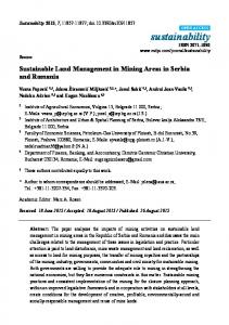
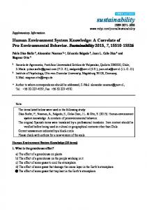
Based on the field operations needed for each crop described in Organic Farm Management Handbook [35], the resource use in terms of fuel and machinery was modeled according to resource use per unit process [38] (see Supplementary Material for detailed description of the farming model). The approach for determining yields and resource use was similar to a previous study commissioned by Defra [39]. 4.2. Model Distribution System The model distribution system from farm gate to consumer’s door was modeled on a crop by crop basis based on published LCA reports for supermarket based food distribution chains [40–42] (Table 3). The chain is thus assumed to consist of 200 km transport to and storage for 5 days at regional distribution center (RDC), 50 km transport to and storage for 2 days at retailers and 6.4 km transport from the retailer to the customer’s home [40] (see Supplementary Material for detailed assumptions.) Transportation from the farm to the RDC is assumed to be in a chilled 32 t truck with an energy consumption of 22.9 mL diesel per euro pallet kilometer [41]. Throughout the system, food waste is taken into account for each crop [42]. The total expenses to labor, service and materials throughout the supply system were estimated based on 12 month average supermarket prices (from March 2012 to March 2013) for each of the vegetables [43]. The prices were adjusted for inflation to reflect average 2009–2010 prices according to the price index for vegetables including potatoes and tubers [44]. 5. Results of Sustainability Assessment The service provided by the three systems is a comparable “basket” of vegetables produced during one year and delivered to the consumer’s door. This service is measured in food energy and is equal to 74,328 MJ/year as an average of 2009 and 2010 (Table 1). This corresponds to the total annual food energy needed for 19–23 people (based on a recommended daily intake of 8.8–11 MJ [45]). The emergy flows are illustrated for the case (Figure 1A) and for the model systems (Figure 1B). The two diagrams demonstrate clearly the different distribution systems and that in the case the full money flow goes to the farm whereas in the model systems part of money flows to the freight companies, supermarkets, and regional distribution centers (RDC). 5.1. Empirical System The basis of any emergy assessment is the emergy table (Table 4) that shows all environmental and societal flows, which support the system. Notably labor and services (L&S) make up 89% of total emergy used by the case (calculated from Table 4). As emergy use for L&S is calculated as a function of the emergy use for the national economy, this reflects the national resource consumption rather than the specific business. To avoid distorting the results of the actual farm with the implications of being embedded in an industrialized economy, we consider the emergy indicators both with and without L&S. The main result of the emergy evaluation for the case system is the transformity of the vegetables, which amounts to 5.20 × 106 seJ/J with L&S and 5.54 × 105 seJ/J without (Table 5). The Emergy Yield Ratio (EYR) of 1.15 disregarding L&S shows that free local environmental services (R) contribute


1921

with only 0.15 seJ per seJ invested from the society. The renewability indicator shows that the system uses 13% local resources when disregarding L&S but only 1% when including L&S. The latter reflects that L&S is considered as non-renewable. Figure 1. Material and emergy flow diagrams for the case system (1A) and the two model systems M-Low and M-High, which have identical distribution systems (1B).

1A

M F L&S £

Sun, wind, rain, geothermal heat

R

Vegetable production

Farm storage

Storage at neighborhood rep.

Van

Foot or bike to home

U

Functional Unit

1B

M L&S

F

National transport system £ Sun, wind, rain, geothermal heat

R

Vegetable production

Farm storage

HGV

Regional distribution center

HGV

Super markets

Car

U

Functional Unit Food waste

Legend:

R = local renewable flows given by the area of the farm, M = fuels and other goods consumed, L&S = direct and indirect labour, F = M+L&S, U = total flow of emergy used for the yearly production and distribution of vegetables to the consumer’s door. HGV = heavy goods vehicles. Functional unit = vegetables in the same quantity at the consumer’s door (74,328 MJ food energy) as the case and of comparable quality as the case (Table 1). Flow limited source

Source

Producer

Storage

Interaction

Transaction

Miscellaneous

Emergy flow Money flow

Disregarding L&S, the emergy profiles of the case system are as follows (calculated from Table 4). Purchased miscellaneous materials for the cultivation phase contribute 38% of total emergy used. Fuel used for cultivation and electricity used for production of seedlings are the biggest flows with 18% and 11%, respectively. Notably, irrigation contributes 24% of the total flow with the water used constituting the most important element (17%). Likewise, the woodchips, used as soil enhancement and used to produce potting compost, contribute with 10% and farm assets contribute with 7%. The diesel used on the weekly round-trip was estimated to 465 L/year (1.6 × 1010 J, Table 4) and it is the major component of the emergy used in the distribution phase (7% of the total emergy used).


1922

Table 3. Outputs and energy use in model distribution system: from farm to regional distribution center (RDC), to retailer and to consumer’s home. Farm

Diesel use,

El. use, 5

RDC

Diesel use,

El. use,

NG use,

Retail

Gasoline use,

Diesel use,

gate

transport to

days storage

gate

transport to

storage at

storage at

gate

transport to

transport to

output

RDC

at RDC

output

retailer

retailer

retailer

output

home by car

home by bus

a

b

(t)

(L)

(kWh)

(t)

c

(L)

a

(kWh)

d

(MJ)

d

(t)

c

(L)

e

(L) e

Potatoes

16.7

64.6

63.9

11.8

11.5

78.1

346.5

11.5

101.2

2.7

Carrots

6.2

24.0

23.7

4.4

4.3

29.0

128.7

4.3

37.6

1.0

Cabbages

5.3

78.3

77.5

5.3

19.6

34.7

591.7

5.1

45.4

1.2

Cauliflower

3.7

55.4

54.9

3.7

13.9

24.5

419.0

3.6

32.1

0.9

Parsnips

2.1

8.1

8.0

1.5

1.4

9.8

43.5

1.4

12.7

0.3

Beetroots

3.5

13.8

13.6

2.5

2.4

16.6

73.8

2.4

21.6

0.6

Onions

3.5

16.8

16.6

3.2

3.8

21.2

115.6

3.2

28.1

0.8

Leeks

2.9

42.5

42.1

2.9

10.6

18.8

321.7

2.8

24.7

0.7

Squash

2.5

37.7

37.3

2.5

9.4

16.7

285.2

2.5

21.9

0.6

Zucchini

6.1

91.5

90.5

6.1

22.9

40.5

691.4

6.0

53.0

1.4

Lettuce

10.4

219.2

216.9

10.1

53.6

66.8

1620.1

9.9

87.6

2.4

Total

62.9

651.8

645.0

54.0

153.3

356.7

4637.2

52.7

465.9

12.6

a

The produce is transported 200 km to RDC and 50 km from RDC to retail [40] using 22.9 ml diesel per pallet-km (chilled single drop, 32 t artic) [41]. b Electricity

consumption in RDC is 0.00059 kWh/l/day [40]. c For each crop losses in storage and packaging are taken into account [42]. See Supplementary Material for details. d

Storage at ambient temperature. Energy use is 0.027 MJ/kg/day (44% electricity for light and 56 % natural gas (NG) for heating) [40]. e Based on an average UK

shopping trip of 6.4 km with an average shopping basket of 28 kg and where 58% of trips made by private car and 8% made by bu s [40]. See Supplementary Material for details.


1923

Table 4. Use of emergy per functional unit for the three systems: the case, M-Low and M-High. See Tables A3 and A4 for notes with details for each item. Unit

Case

M-Low

M-High

UEV

(Unit)

(Unit)

(Unit)

(seJ/unit)

1.0 a

Case emergy

M-Low

M-High

flow

emergy flow

emergy flow

(×1014 seJ)

(×1014 seJ)

(×1014 seJ)

1.0

1.4

0.7

44.0

62.6

29.8

2.5 ×10

9.7

13.8

6.5

1.2 ×104 b

10.8

15.4

7.3

54.8

78.0

37.1

LOCAL RENEWABLE FLOWS (R) 1 2

Sun Evapotranspiration

J

9.7 ×1013

1.4 ×1014

6.6 ×1013

g

3.0 ×10

10

4.3 ×10

10

2.1 ×10

10

11

5.5 ×10

11

2.6 ×10

11

3

Wind

J

3.9 ×10

4

Geo-thermal heat

J

9.0 ×1010

1.3 ×1011

6.1 ×1010

5b

1.5 ×10

3c

SUM (excluding sun and wind) PURCHASED MATERIALS (M) Cultivation Phase Miscellaneous materials 5 6 7 8 9 10

Diesel, fields Lubricant and grease LPG Fleece and propagation tray Electricity Seedlings

J

4.0 ×1010

2.7 ×1010

1.5 ×1010

1.8 ×105 d

73.0

48.9

27.4

J

1.9 ×10

9

1.1 ×10

9

5.7 ×10

8

5d

3.5

2.1

1.0

J

9.1 ×10

8

6.6 ×10

9

2.3 ×10

9

5d

1.7 ×10

1.6

11.3

3.8

g

8.8 ×103

1.9 ×105

9.8 ×104

8.9 ×109 e

0.8

16.7

8.7

J

1.6 ×1010

3.8 ×109

3.8 ×109

2.9 ×105 f

45.4

10.9

10.9

3.2 ×10

5

1.8 ×10

5

9g

0.0

31.0

17.0

2.9 ×10

4

1.3 ×10

4

pcs

0.0 4

11

Seed

g

2.1 ×10

12

Potato seeds

g

1.1 ×106

3.1 ×106

1.3 ×106

1.8 ×10

9.6 ×10

9h

1.5 ×10

0.3

0.4

0.2

2.9 ×109 i

30.1

89.4

37.3

154.6

210.7

106.3

27.8

1.2

0.8

2.9 ×10

0.0

36.9

25.9

1.1 ×106 j

41.5

34.5

24.2

6j

30.8

0.0

0.0

100.0

72.6

50.9

SUM Irrigation 13

Diesel

J

1.5 ×1010

14

Electricity

J

0.0

15

Ground water

g

3.6 ×109

g

9

16

Tap water

1.4 ×10

6.6 ×108

4.6 ×108

1.8 ×105 d

10

9

5f

1.3 ×10

3.0 ×109 0.0

8.9 ×10

2.1 ×109 0.0

2.3 ×10

SUM Soil fertility enhancement 17 18 19 20 21

Woodchips Lime Nitrogen (N) Phosphorus (P2O5) Potash (K2O)

J

3.7 ×1011

0.0

0.0

1.1 ×104 k

38.8

0.0

0.0

g

4

0.0

0.0

1.7 ×109 k

0.3

0.0

0.0

10 l

0.0

0.0

105.7

10 l

0.0

27.1

59.3

g g g

2.0 ×10 0.0

18

0.0 6.6 ×10

4

3.0 ×10

4

2.5 ×10

5

2.8 ×10

4

7.4 ×10

4

2.9 ×10

5

4.1 ×10 3.7 ×10

9k

2.9 ×10

SUM

2.3

8.4

9.8

41.5

35.6

174.8

Farm Assets 22 23

Tractors Other machinery

g

1.4 ×105

8.2 ×104

3.8 ×104

8.2 ×109 m

11.7

16.6

5.8

g

1.5 ×10

5

2.5 ×10

5

1.3 ×10

5

9m

8.0

11.4

5.4

3

8.9 ×10

3

8.9 ×10

3

9e

8.9 ×10

0.8

0.8

0.8

1.1 ×104 k

1.0

1.0

1.0

9e

2.8

0.0

0.0

9e

5.8

0.0

0.0

24

Irrigation pipe

g

8.9 ×10

25

Wood for buildings

J

9.9 ×109

g

7.6 ×10

4

1.9 ×10

4

2.5 ×10

4

26 27 28

Glass for buildings Plastic for buildings Steel for buildings SUM

g g

9.9 ×109 0.0 0.0 0.0

9.9 ×109 0.0 0.0 0.0

5.3 ×10

3.6 ×10 8.9 ×10

9n

3.7 ×10

0.9

0.0

0.0

30.9

29.8

12.7


1924 Table 4. Cont. Unit

Case

M-Low

M-High

UEV

(Unit)

(Unit)

(Unit)

(seJ/unit)

Case emergy

M-Low

M-High

flow

emergy flow

emergy flow

(×1014 seJ)

(×1014 seJ)

(×1014 seJ)

Distribution Phase q 29

Diesel

J

1.6

2.8 ×1010

1.8 ×105 d

28.6

50.3

10

5d

30

Gasoline

J

0.0

1.6 ×10

1.9 ×10

0.0

29.6

31

Electricity

J

0.0

3.6 ×109

2.9 ×105 f

0.0

10.5

0.0

9

4d

0.0

3.2

10 o

1.4

0.0

32 33 34

Natural Gas

J

Machinery (van)

km

Machinery (truck)

5.7 ×10

tkm

4.6 ×10 3

6.8 ×10

0.0

0.0

1.5 ×10

2.5 ×10 4

9p

4.1 ×10

SUM 35

LABOR AND

8.7 ×104

£

SERVICE (L&S) q

1.5 ×105

4.0 ×1012 f

0.0

0.6

30.0

94.2

3451.1

5,854.9

SUM Purchased materials (M)

357.0

442.9

439.0

SUM Feedback from economy (M + L&S)

3808.2

6297.8

6293.9

TOTAL EMERGY USED (U) with L&S

3863.0

6375.8

6330.9

411.9

520.9

476.1

TOTAL EMERGY USED (U) without L&S a

b

c

By definition, Odum (2000) [46], Odum (2000) [47], Brown et al (2011) [48], Buranakarn (1998) [49],

f

NEAD database [50],

h

Coppola (2009) [51], i This study, based on total M-High emergy use (less emergy for distribution phase

g

d

e

This study. Based on input of 20 cm3 peat and 1/774 l diesel per seedling [31],

and seed potato), allocated based on the yields and share of cultivated area used for main crop potato, j

Buenfil (1998) [52],

k

Odum (1996) [23], l Brandt-Williams (2002) [53],

m

Kamp (2011) [54],

n

Bargigli

(2003) [55], °This study. Weight of vehicle: 1500 kg, lifetime 500.000 km and same transformity as for tractors,

p

This study. Transformity per tkm calculated based on Pulselli (2008) [56].

q

M-Low and M-High

have identical distribution system and need the same L&S calculated based on the consumer prices.

Table 5. Emergy indices for the case system, M-Low and M-High with and without labor and service. With labor and service Without labor and service Case M-Low M-High Case M-Low M-High Emergy Yield Ratio (U/F) 1.01 1.01 1.01 1.15 1.18 1.08 Renewability (R/U) 1% 1% 1% 13% 15% 8% 6 6 6 5 5 Solar transformity (seJ/J) 5.20 × 10 8.58 × 10 8.52 × 10 5.54 × 10 7.01 × 10 6.40 × 105

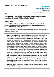
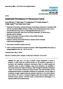
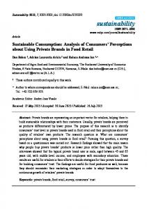
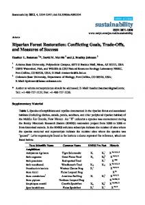
Analyzing the case system using the LCA perspective, the processes related to the cultivation phase have a much larger environmental impact than the processes involved in the distribution phase, for all nine categories (Figure 2). The LCA impact category non-renewable resource use includes all direct and indirect use of fossil and nuclear fuels converted to MJ. Crude oil in the ground contributes more than 50% of the total raw materials for energy (Figure 3). Crude oil is used to produce diesel for operating tractors and pumping the water for irrigation, and to a smaller extent for the manufacture and transport of other inputs.

Sustainability 2014, 6 Figure 2. LCA results for the case, M-Low and M-High for the nine impact categories considered. Impacts per functional unit are divided into distribution phase and cultivation phase.

1925


1926

Figure 3. Contribution of raw materials to the overall result for the Life Cycle Impact category non-renewable resource use (fossil and nuclear) per functional unit for the case, M-Low and M-High.

5.2. Benchmarking Against Model Systems An important difference between the food supply system of the case study and the model systems is the amount of food lost. The long chain in the model systems generates a high percentage of food loss, up to 29% for root vegetables [42]. The direct marketing of the case system implies that the crop loss is smaller due to higher acceptance of less-than-perfect crops. Therefore, the case farm does not need to produce as much to provide the same amount of vegetables at the consumer’s door as the model production system. Land required for providing the food service using standard practices vary between 4.29 ha for the high-yielding model system to 9.02 ha for the low-yielding model system (Table 2). The area required by the case farm (6.36 ha) is within this range. The land use efficiency at the system level may be calculated as the food energy provided to the consumer per hectare of cultivated area (Table 2, vegetables + green manure). This value is 13.3 GJ/ha for the case farm and varies between 9.4 GJ/ha (M-Low) and 19.8 GJ/ha (M-High) for the model systems. This indicates that the case farm has yields within the range of the standard practices. The consumer price of total output from the case system is £86,800. This is significantly lower than the consumer price for the model systems’ output, which is £147,300 (Table 4). That the case farmer is able to sell the products at a significantly lower price may be explained by the fact that the full revenue goes directly to the farm (Figure 1A) whereas in the modeled systems the supermarkets, freight companies and regional distribution centers (RDC) need to make a profit as well (Figure 1B). 5.2.1. Benchmarking Based on Emergy Use The emergy use for purchased materials in the model systems is very similar in total but is differently distributed among the different components, e.g., M-Low has twice as much input in the cultivation phase whereas M-High has five times higher input for soil fertility enhancement. By definition, the emergy use in the distribution phase and for L&S is identical for the two systems. The L&S constitute by far the biggest contribution for both M-Low and M-High with about 92% in both systems. The total emergy used for L&S is 5.9 × 1017 seJ for the model systems (Table 4), which is


1927

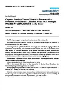
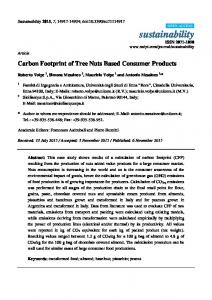
70% more than for the case system. This directly reflects that consumer price for the vegetables are 70% higher in the supermarket than in the direct marketing scheme. When disregarding L&S, the case system uses less emergy to produce the total amount of vegetables sold compared to both model systems (Figure 4). This is especially due to a reduced emergy need for purchased seedlings and seed potato as compared to M-Low and a reduced emergy use for soil enhancements as compared to M-High. In addition, the case distribution system only use one third of the emergy used by the model supply chain. However, the case has a substantial higher consumption of on-farm fuel use and needs more emergy for water for irrigation (Figure 4). Figure 4. Emergy profiles without L&S for the case, M-Low and M-High.

The case-study farm uses significantly more diesel in the cultivation phase (Table 4). This may partially be explained by the tractors being less efficient than those assumed for the model systems. Another factor is that the diesel use per area is more or less independent of the yields, which means that high yielding crops tend to use less fuel per unit output. This is clearly reflected in the comparison of M-Low and M-High, but does not explain why M-Low uses less diesel than the case system. On-farm electricity use (Figure 4) consists of electricity use for on-farm production of seedlings and offices (only for the case-study) as well as for irrigation (only model farms). Disregarding electricity for irrigation, the case uses significantly more electricity than the model systems. However, the electricity consumption of 4350 kWh is still relatively small as it corresponds to the average UK household (4391 kWh, [57]). The emergy needed for electricity in the case system (4.5 × 1015 seJ) is partly compensated by the emergy needed for purchased seedlings in M-Low (3.1 × 1015 seJ) and M-High (1.7 × 1015 seJ) (Table 4). The fact that 30% of the seed potatoes are farm-saved in the case system results in a considerable emergy saving as compared to both model systems. M-Low is particularly bad in this respect since it needs a larger area (Table 2) and thus more seed potatoes to produce the required amount of potatoes (Table 4). M-High has the lowest emergy use for irrigation with M-Low using 50% more and the case using twice as much. The latter is in the first place a consequence of that the case uses more water (3.6 × 109 g groundwater and 1.4 × 109 g tap water) (Table 4). As the annual variation in precipitation is not considered in the model systems, the higher use of water for irrigation in the case system may reflect that the studied period, 2009–2010, was relatively dry, and for instance in 2008 the water use was 70%


1928

less. In addition, tap water, which accounts for 28% of total water used, has an UEV value twice as high as ground water due to the extra work that is needed for pumping and treatment (Table 4). Emergy used for soil enhancement is the biggest input to M-High (Table 4). With 1.7 × 1016 seJ it is more than four times higher than the other systems. This reflects that fertilizer is a valuable resource, and that reducing the import of fertilizer is a key element in reducing emergy use in agricultural systems. The model supply chain needs a total of 805 L diesel (calculated from Table 3) for HGV-transport. In addition, 932 L of gasoline is used for the 58% of the shopping trips done by car and 12.6 L of diesel for the 8% of the trips done by bus. The total use of liquid fuels in the model supply chain (4.5 × 1010 J) is thus bigger than on-farm use of diesel in the cultivation phase in all three systems (Table 4). The total emergy use for the distribution system is three times higher for the model systems than for the case system. M-Low has the largest contribution of local renewable flows as these are calculated directly from the size of the farm (Table 4). Further, the emergy indices (Table 5) reveal that, disregarding L&S, M-High has the smallest share of local renewable inputs (8%). The renewable resources contribute only with 0.08 seJ per seJ invested from society (EYR = 1.08). M-low is in this respect a bit better than the case. The case on the other hand provides the vegetables with the highest resource efficiency (lowest UEV or transformity) and is as such overall more efficient than both model systems (Table 5). This is especially true when also considering L&S in which case the transformity of the case is 39% lower than for M-High. 5.2.2. Benchmarking Based on LCA The distribution phase has an important contribution to the environmental impacts of the model systems and in particular for the impact categories non-renewable resource use, Global Warming Potential (GWP) and human toxicity (Figure 2). The use of non-renewable resources in the case system is similar to M-Low, while the impact of M-High is around 30% lower (Figure 2). The GWP of the case is about 40% higher than both model systems. The difference in GWP between M-Low and the case was related to differences in management processes. The on-farm production of seedlings and composting of woodchips, respectively, may not be as efficient as centralized production of seedlings and use of only green manure and rock phosphate for nutrient supply. The impact category Phosphorus use was calculated to be higher in the case-study as compared to the model systems due to the use of vermiculite, but it is necessary to bear in mind that the levels of phosphorus use were relatively low for all three analyzed systems. The case system and M-Low have significantly lower aquatic eutrophication N potential, terrestrial ecotoxicity and aquatic ecotoxicity than M-High. This is because these impact categories are more dependent on the applied fertilization and irrigation levels rather than on capital goods and on-farm diesel and electricity. Aquatic ecotoxicity and human toxicity effects of the case were also lower than both model systems. Aquatic ecotoxicity levels were found to be similar for model systems while human toxicity of M-Low was shown to be slightly higher than M-High. In addition, for model systems, environmental impacts for all impact categories are clearly dominated by agricultural cultivation (Figure 2). As for the case-study farm, more than 50% of the non-renewable resource use in the model systems is from use of crude oil (Figure 4). Nearly 20% of non-renewable resource use in model systems comes from natural gas, while for the case it is only 10%. Uranium ore has a relatively high contribution, nearly 20% of the result for all systems, as the


1929

electricity mix in the UK includes nuclear energy. Hard coal contributes to around 9% of the resource use and the remaining raw materials play a minor role (5% or less). Assessment of environmental impacts exclusively from the distribution phase reveals that the local distribution system provides significantly lower environmental impacts per functional unit for all of the impact categories considered (Table 6). The relative advantage of the case system compared to the model system reached from 69% for the non-renewable resource use up to 98% in the case of human toxicity potential. Table 6. Environmental impacts per functional unit exclusively for the distribution phase (the same for M-Low and M-High). Impact Category Non-renewable, fossil and nuclear GWP 100 Acidification, GLO Eutrophication aq. N, GLO Eutrophication aq. P, GLO Human toxicity Terrestrial ecotoxicity Aquatic ecotoxicity Phosphorus

Unit MJ eq kg CO2 eq m2 kg N kg P HTP TEP AEP kg

Case Distribution 23,783 1629 92 0.73 0.00 122 2 513 0

Model Distribution 75,923 4890 469 3.74 0.05 6646 21 1445 0

Relative Advantage of Case System (%) 69 67 80 81 91 98 92 64 71

6. Discussion 6.1. LCA versus Emergy Assessment—Handling of Co-Products The assessment of sustainability of the organic low-input vegetable supply system using emergy accounting and LCA has shown that the two methods lead to the same conclusion regarding the supply chain but differ to some extent in the assessment of the production systems. The sometimes contradictory results of the emergy and LCA results are to a large part due to differences in how coproducts, e.g., manure, are accounted for. In emergy accounting, the focus is on the provision of resources, and a key principle in emergy algebra is that all emergy used in a process should be assigned to all co-products as long as they are considered in separate analyses [23]. As manure cannot be produced without producing meat and milk, the entire input to livestock production should be assigned to each of the three products. We have used this approach despite its disadvantages when comparing systems with or without inputs of manure [58]. As a proxy for the UEV of manure, we have combined the UEVs of mineral N, P and K. In the LCA approach, all environmental impacts from animal production were assigned to the main products of animal production being meat and milk. As a result, only emissions associated with transportation, storage and application are considered and the principle of no import of manure in the case system is only partially reflected in the LCA results. Further, this approach has lead to the counter-intuitive result that M-Low has higher phosphorus use than M-High (Figure 2) even though the latter system imports twice as much phosphorus as the former (Table A2). The assumption that manure is a waste may not reflect the actual situation for many organic growers who experience that the supply of N is often a limiting factor for maintaining productivity [59].


1930

6.2. Potentials for Reducing Resource Use in the Case System Even though the case has a strong focus on minimizing use of purchased resources (M), their contribution is still more than six times larger than the contribution from local renewable resources (R) (Table 4). Disregarding L&S, then the largest potential for improving percentage of renewability is to reduce the amount of used fuels (Figure 2). However, to substitute fossil fuelled machinery with more labor intensive practices such as draft animals or manual labor, would under current socio-economic conditions increase overall resource consumption due to the high emergy flow associated with labor. In addition, draft animals would require that a considerable amount of land should be used for feed production. Ground and tap water used for irrigation constitutes 17% of the total emergy use. Due to the differences in UEV between tap and ground water, the emergy use could be substantially reduced by using only ground water. Producing the woodchips, which accounts for 10% of the total emergy used, within the geographical boundaries of the farm would improve renewability. Currently they are residuals supplied from a local gardener who prunes and trims local gardens. In a larger perspective, there are, thus, few environmental benefits from becoming self-sufficient with wood chips in the case system. According to the LCA analysis, the composting process accounts for 30% of greenhouse gas emissions, and using less wood chip compost would reduce the overall global warming potential. Electricity, which is primarily used for heating and lighting in the production of seedlings, constitutes 11% of the emergy used. It is no doubt convenient to use electricity for heating, but substituting the electricity with a firewood based system would largely reduce the emergy. Alternatively, it may be worthwhile to consider harvesting excess heat from the composting process to heat the green house. As for the distribution phase, the case has the potential for decimating fossil fuel consumption by replacing the current customers with some of the many households located within few kilometers of the farm. This could dramatically reduce the 70 km round trip each week. The current way of organizing the distribution, however, is extremely efficient when compared to the alternative where customers would go by car each week and pick up the produce. The latter solution would require up to 1,000,000 car-km per year based on the case farmer’s calculation. With a fuel efficiency of 15 km/L this translates to 66,666 liter of fuel. This is almost 40 times the fuel consumption for the model system (1737 L). 6.3. Outlook for Emergy Use for L&S In a foreseeable future with increasing constraints on the non-renewable resources [6,60], which currently are powering the society with very high EYR-values [23], it is desirable or even necessary that agricultural systems become net-emergy providers, i.e., that more emergy is returned to society from local renewable resources than the society has invested in the production [61]. This requirement means that the contribution from R has to be bigger than F. Bearing in mind that R cannot be increased as the local renewable flows are flow limited, then achieving this can alone be achieved by reducing the emergy currently invested from society, F (3808.2 × 1014 seJ) to less than R (54.8 × 1014 seJ), i.e., by a factor of 70. Such an improvement seems out of reach without transforming the food supply system. Some improvements can be made on the farm as indicated, but the largest change will need to be in the society which determines the emergy use per unit labor. It is important to note that for the standard practices represented by the model system much larger reduction would be required.


1931

Emergy used for L&S accounts for 89% of total emergy flow and constitutes by far the biggest potential for improvements. The L&S-component reflects the emergy used to support people directly employed on the farm and people employed in the bigger economy to manufacture and provide the purchased inputs. Due to the high average material living standard in UK with emergy use per capita being 8.99 × 1016 seJ/year [50], labor is highly resource intensive. Emergy used for L&S can be reduced by reducing the revenue, but this is highly undesirable. Nevertheless, the employees already have a relatively low salary, which they accept because of the benefits enjoyed, e.g., free access to vegetables, cheap accommodation on the farm perimeter and in their opinion a meaningful job close to nature. Thus, the case system attracts people with a Spartan lifestyle with few expenses and thus below average emergy use. In future, it is almost certain that the nation-wide emergy use per capita will be reduced. A likely future scenario for the UK is that the indigenous extraction of non-renewable resources continues to decline (down 23% from 2.4 × 1024 seJ in 2000 to 1.8 × 1024 seJ in 2008 [50]). This is a result of the oil extraction plunging from 2.6 to 1.5 million barrels per day (mbd) from 2000 to 2008 (in 2010 further down to 1.1 mbd) [62]. In the same period the extraction of natural gas dropped from 97.5 to 62.7 million tonnes oil equivalent (and to 40.7 by 2010) [62]. This decline has been compensated by increasing imports of fuels from 57 × 1022 seJ in 2000 to 95 × 1022 seJ by 2008 [50]. The UK has been able to maintain a high level of emergy use per capita by gradually substituting the decline in oil and gas production with imported fuels and services. Such a substitution may continue for some years, but in a longer time perspective a decline in global production of oil, gas and other non-renewable resource is inevitable. Coupled with an increased competition from a growing global population increasing in affluence, it is likely that the import of such resources will eventually decline for the UK as well as other industrialized nations [63]. Such a future scenario imply that the resource consumption per capita will be reduced and thereby that the emergy needed for supporting labor is reduced. However, it may also bring along transformations that are more substantial in the organization of the national economy and all its sub-systems, not least the mass food supply system, which at present uses 9% of UK’s petroleum products. In this perspective, the capacity of a system to adapt to changes is a crucial part of its sustainability, and this characteristic is not directly reflected in the quantitative indicators of emergy assessment and LCA. 6.4. Local Based Box-Scheme versus National-Wide Supermarket Distribution—Resilience The supermarket based distribution system has during the previous decades been redesigned according to principles of Just-In-Time delivery (JIT). These principles aim at reducing the storage need and storage capacity at every link in a production chain, such that a minimum of capital investment is idle or in excess at any time. Less idle capital means fewer costs and fewer environmental impacts. While JIT may decrease environmental impacts per unit of produce for the particular system, as long as everything is running smoothly, it may compromise the system’s resilience as it becomes more vulnerable to disturbance and systemic risks. Systemic risks include disruption in infrastructure supplying money, energy, fuel, power, communications and IT or transport as well as pandemics and climate change [64–66]. As can be imagined any disturbance caused by such events may quickly spread throughout the tightly connected network [65,67]. A loss of IT and communication would make it impossible for a national-wide JIT supply system to coordinate


1932

supplies [64]. A loss of money would make it impossible to conduct transactions with customers. A loss of fuel for transportation would results in large bulks of produce being stranded. A loss of power in the RDC would stop the entire chain and retailers would run out of products in a few days. When benchmarking the case-study against the national wide supermarket system, the former may be more resilient than the latter as it is in a better position to handle infrastructure failures. Due to the higher degree of autonomy and fewer actors involved, the case system would be able to work around many events, which could bring the supermarket-based system to a halt. For instance, a loss of money supply could be handled by delaying payments until the system recovers. Loss of fuel would be difficult to overcome, but produce could still be collected on bike or by public transport. However, from the consumer’s point of view, the risks have a different nature. Consumers in the case system are vulnerable to a poor or failed harvest (e.g., caused by flooding, unusual weather conditions or pests). The supermarket supply system would be unaffected by a failed harvest at a single farm because of the large number of producers feeding into the system. However, the crop diversity of the case-study minimizes the risk of a complete harvest failure. 6.5. Limitations of Study—Validity of Model Systems The vegetables produced from the case-study farm have determined the design of the cultivation phase of the two model systems. It is very likely that other model systems would be developed if the systems were optimized for producing any mix of vegetables of certain food energy content but such analyses are outside the scope of this study. However, as the model systems are scale independent the results can be considered as representing the production from larger areas where different farms are producing different crops. Although in many cases the yields will vary from those presented, the high and low yield scenario should capture the range of possible outcomes. For both emergy assessment and LCA the on-farm use of fuel and irrigation resulted in higher impacts for the case-study than for the model systems. This is to a large part due that the model systems are based on standard data for field operations and that annual variation in rainfall is not reflected. This implies that any additional driving of tractors and machinery, that may occur for various reasons in a real farming system are not included. This may result in an underestimation of the actual resource consumption, which real UK organic farms would have needed in the same years under the same conditions. 7. Conclusions The results of the emergy analysis showed that the case study is more resource efficient than the modeled standard practices, and with the identified potential for further reducing the emergy use, the case-study farm can become substantially better. This is especially true when also considering emergy used to support labor and service. The results of the LCA for the cultivation phase were less conclusive as the case had neither consistently more nor consistently less environmental impacts compared to the model systems. However, for the distribution phase, both the emergy assessment and LCA evaluated the case to perform substantially better than model systems. In addition, we have argued that the case may be in a better position to cope with likely future scenario of reduced access to domestic and imported fossil fuels and other non-renewable resources.


1933

The real value of the case study is that it points out that there are alternative ways of organizing the production and distribution of organic vegetables, which are more resource efficient and potentially more resilient. The case-study shows that it is possible to efficiently manage a highly diverse organic vegetable production system independently of external input of nutrients through animal manure, whilst remaining economically competitive. The success of the case system is to a large part due to management based on a clear vision of bringing down external inputs. This vision is generic but the specific practices of the case-study may not always be the most appropriate for a farm to improve its resource efficiency and resilience. For systems in other societal contexts, e.g., farms with livestock and crop production or farms in remote locations, other strategies will be needed. Acknowledgements This study was supported by the EU grant no. KBBE-245058-SOLIBAM. Special thanks go to the case farmer for providing the data and allowing us to perform research at his interesting farm. Further, we acknowledge the contribution from other SOLIBAM participants, specifically Elena Tavella at the University of Copenhagen, who calculated the revenues. Author Contributions The study was designed by Mads V. Markussen in collaboration with all co-authors. Data was collected by Mads V. Markussen and Michal Kulak with assistance from Laurence G. Smith. All data analysis related to the emergy evaluation was done by Mads V. Markussen, and all data analysis related to LCA was done by Michal Kulak. All authors contributed to combining the analyses and interpreting the results. Supplementary Materials Supplementary materials can be accessed at: http://www.mdpi.com/2071-1050/6/4/1913/s1. Conflicts of Interest The authors declare no conflict of interest. Appendix Table A1. Case system output as average of 2009 and 2010 and classes of crops used for establishment of model systems. Avg. output per year (kg)

Food energy density (KJ/100 g) a

Potatoes, main crop

8589

Potatoes, early

2863

Carrots Carrot bunches

Food energy at consumers (MJ) Individual crops

Groups of crops

298

25,597

25,597

298

8532

8532

3575

109

3897

678

109

739

STORABLE CROPS

Carrots total

4635


1934 Table A1. Cont. Food energy at consumers (MJ)

Avg. output per year (kg)


Beetroot

1446

175

2531

Beetroot bunches

994

175

1740

Individual crops

Groups of crops

STORABLE CROPS

Beetroot total

4271

Onions

2927

116

3396

Spring onions

204

116

237

Onion bunches

48

116

55

Parsnips

1439

247

3555

3555

Leeks

2791

104

2902

2902

Squashes

2474

109

2697

2697

Sprout tops

1661

151

2508

White cabbage

2086

105

2190

Kale

140

155

216

Green cabbage

176

105

185

Red cabbage

181

92

166

Black cabbage

75

155

117

Pak Choi

13

58

7

Cauliflower

890

92

819

Swede/rutabaga

476

123

586

Garlic

91

590

536

Sprouting broccoli

345

117

403

Celeriac

489

77

377

Turnips

184

104

191

Kohlrabi

153

104

159

Mooli radish

126

104

131

Savoy

99

92

91

Fennel

51

82

42

Daikon

8

104

9

Onions, total

3688

Cabbage total

5390

Cauliflower and other storable crops, total

3344

FRESH CROPS Sweet corn

811

369

2992

Courgette

1723

81

1396

Broad beans

713

139

991

Beans, French

649

139

902

Tomatoes

988

73

721

Chard and leaf beet

1050

58

609

Salad pack

1214

49

595

Lettuce

825

49

404

Artichokes

245

93

228

Cucumber

391

52

203

Spinach

273

67

183

Mange tout

81

179

145

Pepper

154

81

125


1935 Table A1. Cont. Food energy at consumers (MJ)

Avg. output per year (kg)


Spring greens

193

49

95

Asparagus

84

75

63

Baby spinach

42

67

28

Salad

45

49

22

Rocket

30

49

15

Individual crops

Groups of crops

FRESH CROPS

Fresh crops, total

9718

Total output a

44,736

74,328

74,328

From Souci et al. [68].

Table A2. Applied nutrients and nutrient balances for M-Low and M-High. Total input N-fixation Atmospheric deposits Applied N Applied P Applied K Output in produce

Nutrient balance a

Unit

M-Lowa

M-Highb

kg N kg N kg N kg P kg K kg N kg P kg K kg N /ha kg P /ha kg K /ha

474 198 0 32 241

225 94 261 70 279 242 32 241

54 0 0

90 10 10

M-Low (7.84 ha) applies 270 kg rock phosphate and 725 kg kali vinasse; b M-High (3.76 ha) applies 44.3 t

cattle farm yard manure, 8 kg rock phosphate and 111 kg kali vinasse.

Table A3. Notes for emergy table (Table 4). Parameter 1

M-Low

M-High

Unit

6.34 ×104

9.02 ×104

4.29 ×104

m2

[CD] [SM]

48.7

48.7

48.7

w/m2

[50]

Sun Area Net radiation

3.15 ×10

7

Net radiation

1.54 × 10

9

Total energy

9.74 ×1013

1.39 ×1014

6.59 ×1013

J/year

0.65

0.65

0.65

m/year

[69]

74

74

74

%

[70]

Conversion factor (60 ×60 ×24 × 365)

2

Comments

Reference a

Case

3.15 ×10

7

1.54 ×10

9

3.15 ×10

7

sek/year

1.54 ×10

9

J/year/m2

Rain Rain (average for the region) Evapotranspiration, arable land Water density Total amount = Area × Rain × Water density × Evapotranpiration

3

1000

1000

1000

kg/m

3.04 ×1010

4.32 ×1010

2.05 ×1010

g/year


1936 Table A3. Cont.

Parameter 3

M-Low

M-High

Unit

1.3

1.3

1.3

kg/m3

[69]

0.001

0.001

0.001 m/s

[50]

Wind Air density Drag coefficient Wind speed average 1999

5.3

Time

5.3

3.15 ×10

Energy = Area × Density × Drag

7

5.3

3.15 ×10

7

3.15 ×10

7

sek/year

3.87 ×1011

5.504 ×1011

2.618 ×1011

J/year

[23]

Heat flow per area

45.0

45.0

45.0

mW/ m2

[71]

Heat flow per area

1.42 ×106

1.42 ×106

1.42 ×106

J/m2/year

Total heat flow

9.00 ×1010

1.28 ×1011

6.09 ×1010

J/year

4.03 ×1010

2.70 ×1010

1.52 ×1010

J/year

1.93 ×109

1.13 ×109

5.73 ×108

J/year

[CD] [SM]

9.12 ×108

6.64 ×109

2.26 ×109

J/year

[CD] [SM]

0

168

89

kg/year

[SM]

coefficient × Wind speed3 ×Time 4

Comments

Reference a

Case

Geothermal heat

CULTIVATION PHASE 5

Diesel, fields Quantity used (3.86 ×1007 J/l)

6

Lubricant /grease Quantity used (38.6 MJ/l, 43.1 MJ/kg)

7

LPG/NG—thermal weeding (flaming) Quantity used (45.6 MJ/kg)

8

Fleece

and

propagation

tray

(polypropylene) Propagation tray Quantity used (10 years lifetime)

520

Conversion factor

17

Quantity used 9

1197

496

17

8840

2

m /year

17

1.88 ×10

5

9.74 ×10

[CD] [SM]

2

g/m 4

[72]

g/year

Electricity (not irrigation) Electricity Quantity used Quantity used (3.6 MJ/kWh)

10

4350 1.57 ×10

1044 10

3.76 ×10

1044 9

3.76 ×10

kWh/year 9

[CD] [SM]

J/year

Seedlings Quantity used

322,933

177,577

pieces

[SM]

Sub-table: Seedlings—calculation of UEV Peat

20

cm3/seedling

[31]

Fossil fuels (heating)

1

l/774 seedling

Fossil fuels (heating)

35.86

MJ/774 seedlings

0.11

g/cm3

[73]

17,150

J/g

[74]

Conversion factors Peat. dry matter Peat heating value (average of two values) Input per seedling

Data

UEV

Emergy

Peat

J

37,730

31,920

1.204 ×109

Diesel

J

46,330

181,000

8.386 ×109 9.59 ×109

UEV for seedlings 11

seJ/one seedling

Seed Quantity used

20,595

29,295

13,068

g/year

[SM]



12

Parameter

Case

M-Low

Potatoe seed

1,050,000

3,123,437

M-High

Unit

1,301,432

g/year

M-High emergy flow (less L&S)

4.388 × 1016

- less supply chain and seed potato (to avoid circular reference)

3.446 ×1016

Area grown with main crop potato

0.3

ha

Yield (40 t/ha)

12.5

t/year

Allocation factor (share of area used for maincrop potatoes—0.31/3.76)

0.083

Comments

Reference a [CD] [SM]

2.863 ×109

sej/g

6.55 ×108

4.59 ×108

J/year

[CD] [SM]

3540

2480

kWh/year

[SM]

UEV seed potatoes IRRIGATION 13

Diesel Quantity used (38.6 MJ/l)

14

1.53 ×1010

Electricity Electricity—irrigation

9

J/year

2.11 ×109

g/year

[CD] [SM]

1.35 ×109

g/year

[CD]

100

m3/year

Electricity—irrigation 15

Density Quantity used (fresh chips, 50 %DM) Dry matter

3.88 ×105 3.88 ×10

g/year

1.94 ×10

7

g DM

21

22

[75]

19.0

GJ/t

Wood energy density

1.90 ×104

J/g

Quantity used

3.69 ×1011

J/year

[76]

2.00 ×104

g

[CD]

Lime

Nitrogen 0.00

2.61 ×105

gN

[CD] [SM]

Imported in fertilizer

32.0

70.0

kg P

[CD] [SM]

Converions factor (kg P2O5 per kg P)

2.29

2.29

kg/kg

Quantity used 20

g/m3

7

Wood energy density

Quantity used 19

3.02 ×109

Woodchips Quantity used

18

3.63 ×109

Tap water Quantity used

17

8.93 ×10

Ground water Quantity used

16

1.27 × 10

10

Phosphorus

Quantity used

73.0

160

kg P2O5

Quantity used

7.33 ×104

1.60 ×105

g P2O5

kg K

Potash Imported in fertilizer

66.4

242

279

Conversion factor (kg K2O per kg K)

1.20

1.20

1.20

kg/kg

Quantity used

80.0

292

336

kg K2O

Quantity used

8.00 ×104

2.92 ×105

3.36 ×105

g K2O

1.43 ×105

2.03 ×105

6.78 ×104

g/year

Appendix 2

Tractors Weight loss per year

Weight of the case’s tractors and lifetime. Model systems scaled to cropping area



Parameter 23

M-High

1.51 ×105

2.14 ×105

1.02 ×105

Comments

Reference a

Weight of the case’s non-motorized machinery divided lifetime min 20 years. Model systems scaled to cropped area.

2.23 ×105

g

Estimate lifetime

25.0

years

Weight loss per year

8920

8920

8920

[CD]

g/year

Wood Storage

building,

general,

wood

construction, non-insulated, at farm

170

Lumber needed per m3 house

200

m3 kg/m3

Lumber used for construction of office 3.40 ×104

conversion factor

2.04 ×107

J/kg

75.0

year

Mass depreciation per year

9.23 ×109

[CD]

kg

and storage area

Estimated lifetime of building

26

Unit

Irrigation pipe (HDPE) Total weight of irrigation pipe

25

M-Low

Other machinery Weight loss per year

24

Case

9.23 ×109

9.23 ×109

J/year

Glass Green house 2 (1970—second hand glass—plastic roof) 7*30 m Glass

210

m2

Thickness

5000

m

Density

2400

kg/m3

Glass

2520

kg

Mass depreciation (estimated glass lifetime 50 year)

5.04 ×1004

[CD]

[77]

g/year

Green house 1 (1890—second hand glass—plastic roof) 8 × 10 m Glass

107

m2

Thickness

5000

m

Density

2400

kg/m3

Glass

1280

kg

Mass depreciation (estimated glass lifetime 50 year) 27

2.57 ×104

[CD]

g/year

Plastic Plastic (roof of green houses)

290

m2

Thickness

5000

m

density

950

kg/m3

Plastic

1380

Mass depreciation

2.76 ×10

[CD]

kg 4

g/year

(glass lifetime 50 year)

Polyethylene covers (polytunnels) Size of covers Thickness Density Quantity used

m2

214 1.83 ×10

4

m

950

kg/m3

3.73 ×104

g/year

Lifetime 7 years. This is average use per year



Parameter 28

Case

M-Low

M-High

Unit

Comments

Reference a

Steel Steel part of polytunnels steel arches

84.0

pcs

Steel per arch

50.0

kg

total steel

2500

kg

Lifetime

100

years

2.50 ×104

g/year

Average haulage distance

70.0

Miles/week

Conversion factor

1.61

km/M

Distance per year

5750

km/year

Mileage

8.09

L/100KM

Mileage

12.0

km/L

Fuel use

465

L/year

Mass depreciation per year

Estimated values

DISTRIBUTION PHASE 29

Diesel

Conversion factor Fuel use

30

3.40 ×107 1.58 ×10

818

818

L/year

Diesel use

2.78 ×1010

2.78 ×1010

J/year

466

466

L/year

3.40 ×10

7

3.40 ×10

Gasoline use

1.58 ×1010

1.58 ×1010

J/year

1001

1001

kWh/year

Table 3

J/L

Electricity

3.60 ×10

6

3.61 ×10

9

3.60 ×10

6

J/kWh

3.61 ×10

9

J/year

4.64 ×1009

J/year

Table 3

Natural gas 4.64 ×1009

NG use (Retail)

Table 3

Machinery (van) Weight

1.50 ×1006 8.20 ×10

Lifetime in km

5.00 ×1005 2.46 ×10

g

09

UEV for lorry

UEV per km

10

seJ/g

Same as for tractors

km

Estimated values

seJ/km

Machinery (Truck) Total ton-km by truck

1.53 ×104

1.53 ×104

tkm

Emergy per truck

8.48 ×1016

8.48 ×1016

seJ/truck

[56]

2.07 ×10

7

2.07 ×10

7

tkm

[56]

4.10 ×10

9

4.10 ×10

9

seJ/tkm

Truck lifetime in tkm Emergy per tkm 35

7

conversion factor

Electricity use

34

Table 3

Gasoline

conversion factor

33

J/year

Diesel use

Electricity use (RDC and Retail)

32

J/l

10

Gasoline use

31

[CD]

Calculated from Table 3

Labor and service Consumer price

86,804.5

[CD]


1940

Table A4. Revenue for model system based on supermarket prices. 12 month avg. price (March 2012

Sold to

Total consumer

to March 2013) [43] (£/kg)

consumers (t)

price (£)

Potatoes, main crop (3/4 of potatoes)

£1.11

8.6

9491

Potatoes. Early (1/4 of potatoes)

£1.39

2.9

3986

Carrots

£1.34

4.3

5705

Cabbages

£1.72

5.1

8850

Cauliflower

£2.25

3.6

8173

Parsnips

£2.88

1.4

4145

Beetroots

£3.46

2.4

8444

Onions

£1.32

3.2

4196

Leeks

£4.95

2.8

13,813

Squash

£2.72

2.5

6730

Courgettes

£2.00

6.0

12,003

Lettuce (little gem)

£7.45

9.9

Model systems–Labor and service

Total/Total price index corrected Price index adjustment

£

Reference a

73,872 159.409/147.264

2012

2009

2010

141.1

128.5

132.2

avg 2009–2010

01.1.7 Vegetables including potatoes and tubers (2005 = 1) Em$ratio (2008 data) Converstion factor EM£ratio a

2.10 × 10

130.35 12

0.53 3.98 × 10

12

Sej/$

[50]

USD/GBP

[78]

Sej/£

Numbers in parentheses refer to references in the reference list, [CD] = Collected data, and

[SM] = Supplementary Material.

References 1.

2. 3.

4.

5. 6. 7.

Pelletier, N.; Audsley, E.; Brodt, S.; Garnett, T.; Henriksson, P.; Kendall, A.; Kramer, K.J.; Murphy, D.; Nemecek, T.; Troell, M. Energy Intensity of Agriculture and Food Systems. Annu. Rev. Environ. Resour. 2011, 36, 223–246. Heller, M.C.; Keoleian, G.A. Assessing the Sustainability of the US Food System: A Life Cycle Perspective. Agric. Syst. 2003, 76, 1007–1041. Barnosky, A.D.; Matzke, N.; Tomiya, S.; Wogan, G.O.U.; Swartz, B.; Quental, T.B.; Marshall, C.; McGuire, J.L.; Lindsey, E.L.; Maguire, K.C.; et al. Has the Earth’s Sixth Mass Extinction Already Arrived? Nature 2011, 471, 51–57. Rockström, J.; Steffen, W.; Noone, K.; Persson, A.; Chapin, S.; Lambin, E.; Lenton, T.; Scheffer, M.; Folke, C.; Schellnhuber, H.J.; et al. Planetary Boundaries: Exploring the Safe Operating Space for Humanity. Ecol. Soc. 2009, 14, 1–33. Sorrell, S.; Speirs, J.; Bentley, R.; Brandt, A.; Miller, R. Global Oil Depletion: A Review of the Evidence. Energ. Pol. 2010, 38, 5290–5295. Cordell, D.; Drangert, J.; White, S. The Story of Phosphorus: Global Food Security and Food for Thought. Global Environ. Change 2009, 19, 292–305. Smil, V. Nitrogen and Food Production: Proteins for Human Diets. Ambio 2002, 31, 126–131.

Sustainability 2014, 6 8. 9. 10.

11. 12. 13.

14.

15. 16. 17.

18. 19. 20. 21. 22. 23. 24. 25.

1941

IAASTD. International Assessment of Agricultural Science and Technology for Development, IAASTD; Island Press: Washington, DC, USA, 2009. Defra. Food Industry Sustainability Strategy; Department for Envronment Food and Rural Affairs: London, UK, 2006. Smith, A.; Watkiss, P.; Tweddle, G.; McKinnon, A.; Browne, M.; Hunt, A.; Treleven, C.; Nash, C.; Cross, S. The Validity of Food Miles as an Indicator of Sustainable Development: Final Report; AEA Technology Environment: London, UK, 2005. Coley, D.; Howard, M.; Winter, M. Local Food, Food Miles and Carbon Emissions: A Comparison of Farm Shop and Mass Distribution Approaches. Food Policy 2009, 34, 150–155. Mundler, P.; Rumpus, L. The Energy Efficiency of Local Food Systems: A Comparison between Different Modes of Distribution. Food Policy 2012, 37, 609–615. Cardinale, B.J.; Duffy, J.E.; Gonzalez, A.; Hooper, D.U.; Perrings, C.; Venail, P.; Narwani, A.; Mace, G.M.; Tilman, D.; Wardle, D.A.; et al. Biodiversity Loss and its Impact on Humanity. Nature 2012, 486, 59–67. Østergård, H.; Finckh, M.R.; Fontaine, L.; Goldringer, I.; Hoad, S.P.; Kristensen, K.; Lammerts van Bueren, E.T.; Mascher, F.; Munk, L.; Wolfe, M.S. Time for a Shift in Crop Production: Embracing Complexity through Diversity at all Levels. J. Sci. Food. Agr. 2009, 89, 1439–1445. Bjorklund, J.; Westberg, L.; Geber, U.; Milestad, R.; Ahnstrom, J. Local Selling as a Driving Force for Increased on-Farm Biodiversity. J. Sustain. Agr. 2009, 33, 885–902. Nemecek, T.; Dubois, D.; Huguenin-Elie, O.; Gaillard, G. Life Cycle Assessment of Swiss Farming Systems: I. Integrated and Organic Farming. Agric. Syst. 2011, 104, 217–232. Audsley, E.; Branderm, M.; Chatterton, J.; Murphy-Bokern, D.; Webster, C.; Williams, A. How Low Can We Go? An Assessment of Greenhouse Gas Emissions from the UK Food System and the Scope to Reduce Them by 2050; FCRN-WWF: London, UK, 2009. Cavalett, O.; Ortega, E. Emergy, Nutrients Balance, and Economic Assessment of Soybean Production and Industrialization in Brazil. J. Clean. Prod. 2009, 17, 762–771. Bastianoni, S.; Marchettini, N.; Panzieri, M.; Tiezzi, E. Sustainability Assessment of a Farm in the Chianti Area (Italy). J. Clean. Prod. 2001, 9, 365–373. Rugani, B.; Benetto, E. Improvements to Emergy Evaluations by using Life Cycle Assessment. Environ. Sci. Technol. 2012, 46, 4701–4712. Raugei, M.; Rugani, B.; Benetto, E.; Ingwersen, W.W. Integrating Emergy into LCA: Potential Added Value and Lingering Obstacles. Ecol. Model. 2014, 271, 4–9. Stockfree Organic Services. Avialable online: http://www.stockfreeorganic.net/ (accessed on 19 June 2013). Odum, H.T. Environmental Accounting: Emergy and Environmental Decision Making; John Wiley & Sons, Inc.: New York, NY, USA, 1996. ISO. ISO 14040: Environmental Management—Life Cycle Assessment—Principles and Framework; International Organization for Standardization: Geneva, Switzerland, 2006. Frischknecht, R.; Jungbluth, N.; Althaus, H.; Bauer, C.; Doka, G.; Dones, R.; Hischier, R.; Hellweg, S.; Humbert, S.; Margni, M.; et al. Implementation of Life Cycle Impact Assessment Methods; Swiss Center for Life Cycle Inventories: Dübendorf, Switzerland, 2007; p. 151.

Sustainability 2014, 6 26.

27. 28.

29. 30.

31.

32. 33. 34. 35. 36.

37.

38.

39.

40.

41.

1942

IPCC. Climate Change 2001: The Scientific Basis. In Third Assessment Report of the Intergovernmental Panel on Climate Change (IPCC); Houghton, J.T., Ding, Y., Griggs, D.J., Noguer, M., van der Linden, P.J., Xiaosu, D., Eds.; Cambridge University Press: Cambridge, UK, 2001. Guinée, J.; van Oers, L.; de Koning, A.; Tamis, W. Life Cycle Approaches for Conservation Agriculture; CML Report 171; Leiden University: Leiden, The Netherlands, 2006; p. 156. Nemecek, T.; Freiermuth, R.; Alig, M.; Gaillard, G. The Advantages of Generic LCA Tools for Agriculture: Examples SALCAcrop and SALCAfarm. In Proceedings of the 7th Int. Conference on LCA in the Agri-Food Sector, Bari, Italy, 22–24 September 2010; pp. 433–438. PréConsultants. SimaPro V 7.3.3; PréConsultants: Amersfoort, The Netherlands, 2007. Frischknecht, R.; Jungbluth, N.; Althaus, H.; Doka, G.; Dones, G.; Heck, T.; Hellweg, S.; Hischier, R.; Nemecek, T.; Rebitzer, G.; et al. The Ecoinvent Database: Overview and Methodological Framework. Int. J. LCA 2005, 10, 3–9. Stoessel, F.; Juraske, R.; Pfister, S.; Hellweg, S. Life Cycle Inventory and Carbon and Water Foodprint of Fruits and Vegetables: Application to a Swiss Retailer. Environ. Sci. Technol. 2012, 46, 3253–3262. Patel, M.; Bastioli, C.; Marini, L.; Würdinger, E. Life‐cycle Assessment of Bio‐based Polymers and Natural Fiber Composites. Biopolymers online 2003, doi:10.1002/3527600035.bpola014. Wihersaari, M. Evaluation of Greenhouse Gas Emission Risks from Storage of Wood Residue. Biomass Bioenerg. 2005, 28, 444–453. ISO. ISO 14044: Environmental Management—Life Cycle Assessment — Requirements and Guidelines; British Standards Institution: London, UK, 2006. Lampkin, N.; Measures, M.; Padel, S. 2011/12 Organic Farm Management Handbook, 9th ed.; The Organic Research Center: Hamstead Marshall, UK, 2011. Gerrard, C.L.; Smith, L.; Pearce, B.; Padel, S.; Hitchings, R.; Measures, M. Public goods and farming. In Farming for Food and Water Security; Lichtfouse, E., Ed.; Springer: London, UK, 2012; pp. 1–22. Smith, L.; Padel, S.; Pearce, B.; Lampkin, N.; Gerrard, C.L.; Woodward, L.; Fowler, S.; Measures, M. Assessing the public goods provided by organic agriculture: Lessons learned from practice. In Organic is Life-Knowledge for Tomorrow, Proceedings of the Third Scientific Conference of ISOFAR, Namyangju, Korea, 28 September–1 October 2011; Volume 2, pp. 59–63. Nemecek, T.; Kägi, T. Life Cycle Inventories of Swiss and European Agricultural Production Systems; Ecoinvent report No. 15a; Swiss Centre for Life Cycle Inventories: Zürich and Dübendorf, Switzerland, December 2007. Williams, A.; Audsley, E.; Sandars, D. Determining the Environmental Burdens and Resource Use in the Production of Agricultural and Horticultural Commodities; Final Report to Defra on Project IS0205; Department for Envronment Food and Rural Affairs: London, UK, 2006. Milài Canals, L. LCA Methodology and Modelling Considerations for Vegetable Production and Consumption; Working Papers 02/07; Center for Environmental Strategy (CES), University of Surrey: Guildford, UK, 2007. Tassou, S.A.; De-Lille, G.; Ge, Y.T. Greenhouse Gas Impacts of Food Retailing; Project code: FO405; Defra: London, UK, 2009.

Sustainability 2014, 6 42.

43. 44.

45. 46.

47.

48. 49. 50. 51.

52. 53.

54.

55.

56.

57.

1943

Terry, L.A.; Mena, C.; Williams, A.; Jenney, N.; Whitehead, P. Fruit and Vegetable Resource Maps: Mapping Fruit and Vegetable Waste through the Retail and Wholesale Supply Chain; Project code: RSC-008; WRAP: Cranfield, UK, 2011. Mysupermarket. Available online: http://www.mysupermarket.co.uk/ (accessed on 3 June 2013). UK National Statistics. Price Indices and Inflation: UK National Statistics Publication Hub Available online: http://www.statistics.gov.uk/hub/economy/prices-output-and-productivity/priceindices-and-inflation/index.html (accessed on 30 May 2013). World Food Programme. What is hunger? Available online: http://www.wfp.org/hunger/what-is (accessed on 10 September 2012). Odum, H.T. Folio #2 Emergy of Global Processes. In Handbook of Emergy Evaluation: A Compendium of Data for Emergy Computation; Center for Environmental Policy, University of Florida: Gainesville, FL, USA, 2000. Odum, H.; Mark, B.; Brandt-Williams, S. Folio #1 Introduction and Global Budget. In Handbook of Emergy Evaluation: A Compendium of Data for Emergy Computation; Center for Environmental Policy, University of Florida: Gainesville, FL, USA, 2000. Brown, M.T.; Protano, G.; Ulgiati, S. Assessing Geobiosphere Work of Generating Global Reserves of Coal, Crude Oil, and Natural Gas. Ecol. Model. 2011, 222, 879–887. Buranakarn, V. Evaluation of Recycling and Reuse of Building Materials using the Emergy Analysis Method. Ph.D. Thesis, University of Florida, Gainesville, FL, USA, 1998. National Environmental Accounting Database. Available online: http://cep.ees.ufl.edu/nead/ (accessed on 3 June 2013). Coppola, F.; Bastianoni, S.; Østergård, H. Sustainability of Bioethanol Production from Wheat with Recycled Residues as Evaluated by Emergy Assessment. Biomass Bioenerg. 2009, 33, 1626–1642. Buenfil, A. Emergy Evaluation of Water. Ph.D. Thesis, University of Florida, Ganiesville, FL, USA, 1998. Brandt-Williams, S. Folio #4 Emergy of Florida Agriculture. In Handbook of Emergy Evaluation: A Compendium of Data for Emergy Computation; Center for Environmental Policy, University of Florida: Gainesville, FL, USA, 2002. Kamp, A.; Østergård, H.; Gylling, M. Sustainability Assessment of Growing and Using Willow for CHP Production. In Proceedings from the 19th European Biomass Conference and Exhibition, Berlin, Germany, 6–10 June 2011; pp. 2645–2656. Bargigli, S.; Ulgiati, S. Emergy and Life-Cycle Assessment of Steel Production in Europe. In Emergy Synthesis 2: Theory and Application of the Emergy Methodology, Proceedings from the Second Biennial Emergy Analysis Research Conference, Gainesville, FL, USA, 20–22 September 2001; pp. 141–156. Pulselli, R.M.; Simoncini, E.; Ridolfi, R.; Bastianoni, S. Specific Emergy of Cement and Concrete: An Energy-Based Appraisal of Building Materials and their Transport. Ecol. Ind. 2008, 8, 647–656. Regional and Local Authority Electricity Consumption Statistics: 2005 to 2011. Available online: https://www.gov.uk/government/statistical-data-sets/regional-and-local-authority-electricityconsumption-statistics-2005-to-2011 (accessed on 3 June 2013).

Sustainability 2014, 6 58. 59.

60. 61. 62.

63.

64.

65. 66. 67. 68. 69. 70. 71. 72. 73.

74. 75. 76.

1944

Kamp, A.; Østergård, H. How to Manage Co-Product Inputs in Emergy Accounting Exemplified by Willow Production for Bioenergy. Ecol. Model. 2013, 253, 70–78. Berry, P.M.; Sylvester-Bradley, R.; Philipps, L.; Hatch, D.J.; Cuttle, S.P.; Rayns, F.W.; Gosling, P. Is the Productivity of Organic Farms Restricted by the Supply of Available Nitrogen? Soil Use Manag. 2002, 18, 248–255. Brown, M.T.; Ulgiati, S. Understanding the Global Economic Crisis: A Biophysical Perspective. Ecol. Model. 2011, 223, 4–13. Odum, H.T.; Odum, E.C. The Prosperous Way Down. Energy 2006, 31, 21–32. Statistical Review of World Energy 2012. Available online: http://www.bp.com/assets/bp_internet/ globalbp/globalbp_uk_english/reports_and_publications/statistical_energy_review_2011/STAGING/ local_assets/pdf/statistical_review_of_world_energy_full_report_2012.pdf (accessed on 3 June 2013). UK Ministry of Defense. Regional Survey: South Asia Out to 2040. Strategic Trends Programme. Available online: https://www.Gov.uk/government/uploads/system/uploads/attachment_data/file/ 49954/20121129_dcdc_gst_regions_sasia.pdf (accessed on 3 June 2013). Peck, H. Resilience in the Food Chain: A Study of Business Continuity Management in the Food and Drink Industry: Final Report to the Department for Environment, Food and Rural Affairs; Defra: Shrivenham, UK, 2006; p. 171. Goldin, I.; Vogel, T. Global Governance and Systemic Risk in the 21st Century: Lessons from the Financial Crisis. Global Pol. 2010, 1, 4–15. Fantazzini, D.; Höök, M.; Angelantoni, A. Global Oil Risks in the Early 21st Century. Energ. Pol. 2011, 39, 7865–7873. Korhonen, J.; Seager, T.P. Beyond Eco-Efficiency: A Resilience Perspective. Bus. Strat. Environ. 2008, 17, 411–419. Souci, S.; Fachmann, W.; Kraut, H. Food Composition and Nutrition Tables, 6th ed.; CRC Press: Stuttgart, Germany, 2000. Regional Climates: Southern England. Available online: http://www.metoffice.gov.uk/climate/uk/so/ (accessed on 28 February 2014). Dunn, S.M.; Mackay, R. Spatial Variation in Evapotranspiration and the Influence of Land use on Catchment Hydrology. J. Hydrol. 1995, 171, 49–73. British Geological Survey. Available online: http://www.bgs.ac.uk/research/energy/geothermal/ (accessed on 28 February 2014). Shawbury Garden Center. Gardening Supplies. Available online: http://www.shawburygardencentre.co.uk/ (accessed on 28 February 2014). Brown, M.; Bardi, E. Folio #3 Emergy of Ecosystems. In Handbook of Emergy Evaluation: A Compendium of Data for Emergy Computation; Center for Environmental Policy, University of Florida: Gainesville, FL, USA, 2001. Engineeringtoolbox. Fuels-Higher Calorific Values. Available online: http://www.engineeringtoolbox. com/fuels-higher-calorific-values-d_169.html (accessed on 28 February 2014). Francescato, V.; Antonini, E.; Luca, B. Wood Fuels Handbook; Italian Agriforestry Energy Association: Legnaro, Italy, 2008; pp. 79. Skov-og Naturstyrelsen. Træ som brændsel. Available online: http://skov-info.dk/haefte/18/ kap07.htm (accessed on 28 February 2014). (In Danish)

Sustainability 2014, 6 77. 78.

1945

The Physics Factbook. Density of Glass. Available online: http://hypertextbook.com/facts/2004/ ShayeStorm.shtml (accessed on 28 February 2014). OANDA. Historical Exchange Rates. Available online: http://www.oanda.com/currency/ historical-rates/ (accessed on 28 February 2014).

© 2014 by the authors; licensee MDPI, Basel, Switzerland. This article is an open access article distributed under the terms and conditions of the Creative Commons Attribution license (http://creativecommons.org/licenses/by/3.0/).

Evaluating the Sustainability of a Small-Scale Low-Input ... - MDPI

Evaluating the Sustainability of a Small-Scale Low-Input ... - MDPI

Suggest Documents

Neighborhood Sustainability Assessment: Evaluating ... - MDPI

A Simplified Method for Evaluating Building Sustainability in ... - MDPI

A Simplified Method for Evaluating Building Sustainability in ... - MDPI

Evaluating Sustainability and Democracy in the Development ... - MDPI

EVALUATING THE SUSTAINABILITY OF SUBSISTENCE ... - CiteSeerX

Development of a Framework for Evaluating the Sustainability of ...

Sustainability Management with the Sustainability Balanced ... - MDPI

Sustainability Management with the Sustainability Balanced ... - MDPI

Sustainability - MDPI

sustainability - MDPI

sustainability - MDPI

sustainability - MDPI

sustainability - MDPI

sustainability - MDPI

sustainability - MDPI

sustainability - MDPI

sustainability - MDPI

sustainability - MDPI

sustainability - MDPI

sustainability - MDPI

sustainability - MDPI

sustainability - MDPI

Evaluating sustainability: a retrospective cohort analysis of the ...

Evaluating the Quality of Web Based Sustainability Reports: A Multi ...