Evaluation and Improvement of Two Training Algorithms Tae-Hoon Kim, Jiang Li and Michael T. Manry University of Texas at Arlington Department of Electrical Engineering Arlington, TX 76019 Telephone:(817) 272-3469 FAX: (817) 272-2253 Email:
[email protected] linear transformation of the input vectors, and (3) approach theoretically attainable values of training error, such as Cramer-Rao-MAP bounds [7]. The desired properties of training algorithms are: (P1) The algorithm should work well for both correlated and random data. By correlated data, we mean (a) that inputs and desired outputs are correlated, and (b) inputs may be correlated with each other. (P2) The algorithm should be invariant to input biases and variances. (P3) For large enough networks, memorization should take place during training. Thus, zero is our lower bound on training error. If an algorithm fails to memorize data sets having a small number of patterns, it can be considered to have a problem. The upper bound on pattern storage [6] for a neural net is denoted by N Su = w (2.1) M where the number of network parameters Nw is
Abstract Two effective neural network training algorithms are output weight optimization – hidden weight optimization and conjugate gradient. The former performs better on correlated data, and the latter performs better on random data. Based on these observations and others, we develop a procedure to test general neural network training algorithms. Since good neural network algorithm should perform well for all kinds of data, we develop alternation algorithms, which have runs of the different algorithms in turn. The alternation algorithm works well for both kinds of data.
1. Introduction The Conjugate gradient (CG) algorithm occasionally performs well in artificial neural network (ANN) training [1 – 4]. Another training algorithm, which often performs well, is output weight optimization – hidden weight optimization (OWO-HWO) [5]. Experimentation has shown that CG performs better on random data and OWOHWO performs better on correlated data. Based on these observations, we develop a set of desired training algorithm properties in section 2. In section 3 we show that both algorithms lack some of the desired properties. In section 4 we construct a new algorithm that has all the desired properties. In section 5, we present numerical results. In section 6, we conclude this paper.
Nw = (N+1)Nh + (N+Nh+1)M
for a fully connected MLP, which includes bypass weights. Here N, Nh, and M respectively denote number of inputs, hidden units and outputs.
2.1 Data file types Following properties (P1) and (P3), four kinds of data can be prepared for testing the algorithms. In random data, input and desired output vectors have statistically independent elements, generated by a random number generator. In random memorization (RM) data, the number of training patterns, Nv, satisfies the condition Nv = Su. In random non-memorization (RN) data, Nv >> Su. Correlated training data can take many forms. We assume that elements of the input vector are correlated,
2. Desired training algorithm properties Many investigators have described Multilayer Perceptron (MLP) training algorithm properties, both good and bad. In general it is convenient for the algorithm to: (1) work equally well for all types of data, (2) be invariant to
0-7803-7576-9/02$17.00 © 2002 IEEE
(2.2)
1019
and that correlations exist between input and desired output vector elements. In correlated memorization (CM) data, Nv satisfies the condition Nv = Su. In correlated nonmemorization (CN) data, Nv >> Su.
and the hidden layer delta functions is
2.2 Procedure to evaluate training algorithms
let’s express the input as a sum of the ith input mean mi and a zero-mean input zpi as x pi = z pi + mi (3.3)
M
δ ph ( j ) = O j ⋅ (1 − O j )⋅ ∑ δ po (k ) ⋅ wo (k , N + j + 1)
The proposed steps for evaluating a training algorithm are as follows: Step 1: Determine whether or not the algorithm is invariant to input variances and biases. Invariance is the desired outcome. Step 2: Test the algorithm on RM and RN data. It is desirable that the training error for RM data is much less than the training error of RN data. Step 3: Test the algorithm on CM and CN data. It is desirable that the training error for CM data is much less than the training error of CN data.
In the following, we show why the gradients are different for biased and unbiased training data: (1) Input to hidden weight gradients for the unbiased and biased cases are respectively −∂E p
∂w( j, i)
−∂E p
∂w( j, i ) b
= δ ph ( j ) ⋅ z pi
(
(3.4)
−∂E p
)
= δ ph ( j ) ⋅ z pi + mi =
∂w( j, i )
+ δ ph ( j ) ⋅ mi (3.5)
3. Evaluation of training algorithms
(2) Input to output weight gradients for unbiased and biased cases are respectively
In this section, we evaluate the CG and OWO-HWO training algorithms following the steps above.
−∂E p
∂wo (k , i )
3.1 Evaluation of CG: −∂E p
As an experiment we applied CG to biased and unbiased RM data. The multilayer perceptron (MLP) structure was 8-36-1 and the training error for each case is shown in Fig 1. We see that CG memorized only the unbiased data. In
∂wo (k, i ) b
(
1
= δ po (k ) ⋅ z pi + mi =
−∂E p
0.8
∂wo (k , j )
0.7
−∂E p
MSE
0.6
CG on unbiased data CG on biased data
∂wo (k , j ) b
0.4
−∂E p
∂wo (k, i )
(3.6)
+ δ po (k ) ⋅ mi
= δ po (k ) ⋅ O j
= δ po (k ) ⋅ O j =
−∂E p
∂wo (k , j )
(3.8) (3.9)
From equations (3.4–3.9), we observe that input connected weight gradients for unbiased and biased data are different. Thus the performance of CG is dependent on input biases. A similar result holds for input variances.
0.3 0.2 0.1 0
)
= δ po (k ) ⋅ z pi
(3.7) (3) Hidden to output weight gradients for unbiased and biased cases are respectively
0.9
0.5
(3.2)
k =1
0
200
400
600
800
1000
1200
1400
1600
1800
2000
Iteration number
3.2 Evaluation of OWO-HWO
Fig 1. CG applied to biased and unbiased RM data
In OWO-HWO we alternately, solve linear equations for output weights and solve linear equations for hidden weight changes. Therefore input biases should have no effect on training. In the following, we evaluate OWOHWO training and show how the performance of OWOHWO compares to that of CG on RM and CM data. The RM data set RV369.tra, generated by a random number
the following we show that gradients are affected by biases. Assuming linear output activation, the output layer delta function for the kth output is
δ po (k ) = 2 ⋅ (t pk − y pk )
(3.1)
1020
generator, contains 369 patterns. The MLP structure is 836-1 so that it satisfies Nv = Su. The training error for each algorithm is shown in Fig. 2. We observe that memorization takes place for CG algorithm, but not for
Nv = Su. The training error for each algorithm is given in Fig. 3. We see that OWO-HWO outperforms CG even though both algorithms fail to completely memorize. We want to mention that the target output values in Power14.tra are large hence the resulting MSE is large. Obviously, both algorithms alone cannot satisfy all the desired properties.
0.8
0.7
4. Alternation algorithms
0.6
OWO-HWO CG
MSE
0.5
OWO-HWO and CG have different performance on different types of data, Aiming to satisfy all the desired properties, we need to combine these two algorithms in some way. When one of the algorithms learns slowly, we switch to the other algorithm. Two alternating algorithms, which perform well on all four data types, are developed here.
0.4
0.3
0.2
0.1
0
0
100
200
300
400
500
600
700
800
900
1000
4.1 Fixed Alternation (FA)
Iteration number
Fig. 2: OWO-HWO & CG applied on RM data
This algorithm has fixed If and Ioh throughout the training, where If and Ioh are the numbers of iterations for CG and OWO-HWO applied in each training cycle respectively. A training cycle includes If iterations of CG followed by Ioh iterations of OWO-HWO. In FA case, we set If = Ioh for each training cycle. The numbers If and Ioh are determined heuristically. When a certain number of iterations makes the algorithm get stuck in a local minimum, we use either a bigger or smaller number of iterations.
OWO-HWO, and CG outperforms OWO-HWO. Unbiased CM data set power14.tra is obtained from TU Electric Company in Texas. It has 14 inputs and one output. The first ten input features are the last ten minutes’ average power load in megawatts for the entire TU Electric utility, 8000
7000
4.2 Adaptive Alternation (AA)
OWO-HWO CG 6000
The adaptive alternation algorithm varies the numbers of iterations If and Ioh for each training cycle depending on their performances in the previous training cycle. The algorithm, which has the larger error decrease in the previous training cycle, is given more iterations in the next training cycle. For the first training cycle, we run both algorithms for a fixed amount of iterations and calculate the training error decrease for each algorithm, i.e. Df and Doh. Then If and Ioh for the next training cycle are calculated as follows:
MSE
5000
4000
3000
2000
1000
0
0
50
100
150
200
250
300
350
400
Iteration number
Fig. 3: OWO-HWO & CG applied to CM data
Df I
which covers a large part of north Texas. The output is the forecast power load fifteen minutes in the future from the current time. All powers are originally sampled every fraction of a second, and averaged over 1 minute to reduce noise. We chose the structure 14-10-1 for this data. The original data contains 1768 patterns, we randomly pick 175 patterns so as it satisfies the memorization condition
f
← It ⋅
I
f
D f + D oh
=
2 Df It ⋅ I f D f + D oh
(4.1)
It
I oh
1021
D oh 2 I D oh I oh ← It ⋅ = t ⋅ D f + D oh I oh D f + D oh It
(4.2)
where It is the total number of iterations for both algorithms in the previous training cycle. This process of equations (4.1) and (4.2) goes on until the end of training. An important property of AA is that the computational resources are allocated to the better performing algorithm.
boost tub oscillatory axial load (OAL), lateral cyclic boost tube OAL, collective boost tube OAL, main rotor pitch link OAL, etc. This data was obtained from the M430 flight load level survey conducted in Mirabel Canada in early 1995 by Bell Helicopter of Fort Worth. We chose a 15-17-9 MLP structure for F-17.tra. The input vectors have been replaced by their KLT transformations, which compressed the dimension of the input vectors from 17 to 15. The original data set contains 2823 patterns, in order to meet memorization condition Nv = Su, we randomly picked 63 patterns so as it satisfies equation (2.1). Figure 5 shows that AA performs well. We want to mention that the target output values in F17.tra are large hence the resulting MSE is large.
5. Performance comparisons After running CG, OWO-HWO and AA algorithms on a lot of unbiased training data, we observed that AA performed best in most of correlated training data but second best in random training data. Contrary to what we hoped, AA didn’t perform significantly better than FA. In half of the training data, FA performed a little bit better. Regular switching of the algorithms was enough to let the
18
10000
OWO-HWO CG AA
9000
x 10
6
16
OWO-HWO CG AA
14
12
MSE
MSE
8000
7000
10
8
6
6000
4 5000 2
4000
0
50
100
150
200
250
300
350
0 50
400
100
150
200
250
300
350
Iteration number
Iteration number
Fig 4. Algorithm performance on CN power14.tra
Fig. 5 Algorithm performance on CM F17.tra
algorithm get out of local minimum. In this section, we show typical plots of the comparisons. All the algorithms ran on normalized data, and for some of the data, we used KLT transformations to compress the inputs. First, the algorithms were run on CN data set Power14.tra, which is the original Power14.tra data set with 1768 patterns so as it satisfy non-memorization condition Nv >> Su. The MLP structure is 14-10-1. For AA, an initial training cycle consists of 20 iterations of CG and 20 iterations of OWO-HWO. We can see that AA performs best (Fig. 4). Second, the algorithms were run on CM data set F17.tra, which is for onboard Flight Load Synthesis (FLS) in helicopters. In FLS, we estimate mechanical loads on critical parts, using measurements available in the cockpit. The accumulated loads can then be used to determine component retirement times. There are 17 inputs and 9 outputs for each pattern. In this approach, signals available on an aircraft, such as airspeed, control attitudes, accelerations, altitude, and rates of pitch, roll, and yaw, are processed into desired output loads such as fore/aft cyclic
1
OWO-HWO CG AA
0.9
0.8
MSE
0.7
0.6
0.5
0.4
0.3
0
100
200
300
400
500
600
700
800
900
1000
Iteration number
Fig. 6 Algorithm performance on RN RV1000.tra
Third, the algorithms were run on RN data set RV1000.tra, which is generated by a random generator. It consists of 8 inputs and 1 output, 1000 patterns. All
1022
elements have the same variances and their energies are evenly distributed, so we don’t need to normalize the data. The MLP structure is 8-36-1. From Fig 6 we can see that AA performs second best. Fourth, the algorithms were run on 369 patterns of RM data set RV369.tra. The MLP structure of the network is 836-1. We can see from Fig.7 that AA performs second best.
[3]
[4] [5]
0.8
OWO-HWO CG AA
0.7
0.6
[6]
MSE
0.5
0.4
0.3
[7]
0.2
0.1
0
0
100
200
300
400
500
600
700
800
900
1000
Iteration number
Fig. 7 Algorithm performance on RM RV369.tra
6. Conclusions In this paper we have introduced a set of desired properties for MLP training algorithms and shown that both CG and OWO-HWO alone lack these properties. Alternation algorithms are developed and run on normalized and KLTed data sets. Among the three algorithms, AA works best for correlated data sets and second best for random data sets. We observe that unless some algorithms are specifically suitable for certain kinds of data, AA performs well. We can say that AA algorithm has the desired properties.
Acknowledgment This work was founded by the Advanced Technology Program of the state of Texas under grant 003656-01292001.
References [1]
[2]
J.P. Fitch, S.K. Lehman et al., “Ship wake-detection procedure using conjugate gradient trained artificial neural networks,” Geoscience and Remote Sensing, IEEE Transactions on, vol. 29 Issue: 5, pp. 718-726, Sept. 1991 E.M. Johansson, F.U. Dowla and D.M. Goodman, “Backpropagation learning for multilayer feed-forward neural networks using the conjugate gradient method,”
1023
International Journal of Neural Systems, vol. 2, no. 4, pp. 291-301, 1991. C. Charalambous, “Conjugate gradient algorithm for efficient training of artificial neural networks,” Circuits, Devices and Systems, IEE Proceedings, Vol. 139, Issue: 3, pp. 301–310, June 1992. E. Barnard, “Optimization for training neural nets,” Neural Networks, IEEE Transactions on, Vol. 3, Issue: 2, pp. 232–240, March 1992. H.H. Chen, M.T. Manry and H. Chandrasekaran, “A Neural Network training Algorithm Utilizing Multiple Sets of linear equations,” Neurocomputing, vol. 25, no. 1-3, pp. 55-72, April 1999. A. Gopalakrishnan, X. Jiang, M.S. Chen and M.T. Manry, “Constructive proof of efficient pattern storage in the multilayer perceptron,” Twenty seventh Asilomar Conference on Signals, Systems & Computers, vol. 1, pp. 386-390, Nov 1993. M.T. Manry, Cheng-Hsiung Hsieh, M.S. Dawson, A.K. Fung and S.J. Apollo, "Cramer Rao Maximum APosteriori Bounds on Neural Network Training Error for Non-Gaussian Signals and Parameters," International Journal of Intelligent Control and Systems, vol. 1, no. 3, pp. 381-391, 1996.