Evaluation of Random Subspace and Random Forest Regression Models Based on Genetic Fuzzy Systems Tadeusz Lasota1, Zbigniew Telec2, Bogdan Trawiński2, Grzegorz Trawiński3 1
Wrocław University of Environmental and Life Sciences, Dept. of Spatial Management ul. Norwida 25/27, 50-375 Wrocław, Poland 2 Wrocław University of Technology, Institute of Informatics, Wybrzeże Wyspiańskiego 27, 50-370 Wrocław, Poland 3 Wrocław University of Technology, Faculty of Electronics, Wybrzeże S. Wyspiańskiego 27, 50-370 Wrocław, Poland
[email protected],
[email protected], {zbigniew.telec, bogdan.trawinski}@pwr.wroc.pl
Abstract. The random subspace and random forest ensemble methods using a genetic fuzzy rule-based system as a base learning algorithm were developed in Matlab environment. The methods were applied to the real-world regression problem of predicting the prices of residential premises based on historical data of sales/purchase transactions. The computationally intensive experiments were conducted aimed to compare the accuracy of ensembles generated by the proposed methods with bagging, repeated holdout, and repeated crossvalidation models. The statistical analysis of results was made employing nonparametric Friedman and Wilcoxon statistical tests. Keywords: genetic fuzzy systems, random subspaces, random forest, bagging, repeated holdout, cross-validation, property valuation, noised data
1
Introduction
Ensemble models have been drawing the attention of machine learning community due to its ability to reduce bias and/or variance compared with their single model counterparts. The ensemble learning methods combine the output of machine learning algorithms to obtain better prediction accuracy in the case of regression problems or lower error rates in classification. The individual estimator must provide different patterns of generalization, thus the diversity plays a crucial role in the training process. To the most popular methods belong bagging [2], boosting [23], and stacking [24]. In this paper we concentrate on bagging family of techniques. Bagging, which stands for bootstrap aggregating, devised by Breiman [2] is one of the most intuitive and simplest ensemble algorithms providing good performance. Diversity of learners is obtained by using bootstrapped replicas of the training data. That is, different training data subsets are randomly drawn with replacement from the original training set. So obtained training data subsets, called also bags, are used then to train different classification and regression models. Theoretical analyses and experimental results
proved benefits of bagging, especially in terms of stability improvement and variance reduction of learners for both classification and regression problems [5], [8]. Another approach to ensemble learning is called the random subspaces, also known as attribute bagging [4]. This approach seeks learners diversity in feature space subsampling. All component models are built with the same training data, but each takes into account randomly chosen subset of features bringing diversity to ensemble. For the most part, feature count is fixed at the same level for all committee components. The method is aimed to increase generalization accuracies of decision tree-based classifiers without loss of accuracy on training data. Ho showed that random subspaces can outperform bagging and in some cases even boosting [11]. While other methods are affected by the curse of dimensionality, random subspace technique can actually benefit out of it. Both bagging and random subspaces were devised to increase classifier or regressor accuracy, but each of them treats the problem from different point of view. Bagging provides diversity by operating on training set instances, whereas random subspaces try to find diversity in feature space subsampling. Breiman [3] developed a method called random forest which merges these two approaches. Random forest uses bootstrap selection for supplying individual learner with training data and limits feature space by random selection. Some recent studies have been focused on hybrid approaches combining random forests with other learning algorithms [9], [14]. We have been conducting intensive study to select appropriate machine learning methods which would be useful for developing an automated system to aid in real estate appraisal devoted to information centres maintaining cadastral systems in Poland. So far, we have investigated several methods to construct regression models to assist with real estate appraisal: evolutionary fuzzy systems, neural networks, decision trees, and statistical algorithms using MATLAB, KEEL, RapidMiner, and WEKA data mining systems [10], [15], [16]. A good performance revealed evolving fuzzy models applied to cadastral data [17], [20]. We studied also ensemble models created applying various weak learners and resampling techniques [13], [18], [19]. The first goal of the study presented in this paper was to compare empirically random subspace, random forest, bagging, repeated holdout, and repeated crossvalidation ensemble models employing genetic fuzzy systems (GFS) as base learners. The algorithms were applied to real-world regression problem of predicting the prices of residential premises, based on historical data of sales/purchase transactions obtained from a cadastral system. The second goal was to examine the performance of the ensemble methods with noisy training data. The resilience to noised data can be an important criterion for choosing appropriate machine learning methods to our automated valuation system. The susceptibility of machine learning algorithms to noised data has been explored in several works, e.g. [1], [12], [21], [22].
2 Methods Used and Experimental Setup The investigation was conducted with our experimental system implemented in Matlab environment using Fuzzy Logic, Global Optimization, Neural Network, and Statistics toolboxes. The system was designed to carry out research into machine
learning algorithms using various resampling methods and constructing and evaluating ensemble models for regression problems. Real-world dataset used in experiments was drawn from an unrefined dataset containing above 50 000 records referring to residential premises transactions accomplished in one Polish big city with the population of 640 000 within 11 years from 1998 to 2008. The final dataset counted the 5213 samples. Five following attributes were pointed out as main price drivers by professional appraisers: usable area of a flat (Area), age of a building construction (Age), number of storeys in the building (Storeys), number of rooms in the flat including a kitchen (Rooms), the distance of the building from the city centre (Centre), in turn, price of premises (Price) was the output variable. For random subspace and random forest approaches four more features were employed: floor on which a flat is located (Floor), geodetic coordinates of a building (Xc and Yc), and its distance from the nearest shopping center (Shopping). Due to the fact that the prices of premises change substantially in the course of time, the whole 11-year dataset cannot be used to create data-driven models. In order to obtain comparable prices it was split into 20 subsets covering individual half-years. Then the prices of premises were updated according to the trends of the value changes over 11 years. Starting from the beginning of 1998 the prices were updated for the last day of subsequent half-years. The trends were modelled by polynomials of degree three. The chart illustrating the change trend of average transactional prices per square metre is given in Fig. 1. We might assume that half-year datasets differed from eachother and might constitute different observation points to compare the accuracy of ensemble models in our study and carry out statistical tests. The sizes of half-year datasets are given in Table 1.
Fig. 1. Change trend of average transactional prices per square metre over time Table 1. Number of instances in half-year datasets 1998-2 202 2003-2 386
1999-1 213 2004-1 278
1999-2 264 2004-2 268
2000-1 162 2005-1 244
2000-2 167 2005-2 336
2001-1 228 2006-1 300
2001-2 235 2006-2 377
2002-1 267 2007-1 289
2002-2 263 2007-2 286
2003-1 267 2008-1 181
As a performance function the root mean square error (RMSE) was used, and as aggregation functions of ensembles arithmetic averages were employed. Each input and output attribute in individual dataset was normalized using the min-max
approach. The parameters of the architecture of fuzzy systems as well as genetic algorithms are listed in Table 2. Similar designs are described in [6], [7], [15]. Table 2. Parameters of GFS used in experiments Fuzzy system Type of fuzzy system: Mamdani No. of input variables: 5 Type of membership functions (mf): triangular No. of input mf: 3 No. of output mf: 5 No. of rules: 15 AND operator: prod Implication operator: prod Aggregation operator: probor Defuzzyfication method: centroid
Genetic Algorithm Chromosome: rule base and mf, real-coded Population size: 100 Fitness function: MSE Selection function: tournament Tournament size: 4 Elite count: 2 Crossover fraction: 0.8 Crossover function: two point Mutation function: custom No. of generations: 100
Following methods were applied in the experiments, the numbers in brackets denote the number of input features: CV(5) – Repeated cross-validation: 10-fold cv repeated five times to obtain 50 pairs of training and test sets, 5 input features pointed out by the experts, BA(5) – 0.632 Bagging: bootstrap drawing of 100% instances with replacement (Boot), test set – out of bag (OoB), the accuracy calculated as RMSE(BA) = 0.632 x RMSE(OoB) + 0.368 x RMSE(Boot), repeated 50 times, RH(5) – Repeated holdout: dataset was randomly split into training set of 70% and test set of 30% instances, repeated 50 times, 5 input features, RS(5of9) – Random subspaces: 5 input features were randomly drawn out of 9, then dataset was randomly split into training set of 70% and test set of 30% instances, repeated 50 times, RF(5of9) – Random forest: 5 input features were randomly drawn out of 9, then bootstrap drawing of 100% instances with replacement (Boot), test set – out of bag (OoB), the accuracy calculated as RMSE(BA) = 0.632 x RMSE(OoB) + 0.368 x RMSE(Boot), repeated 50 times. We examined the aforementioned ensemble methods also for their susceptibility to noised data. Each run of experiment was repeated four times: firstly each output value (price) in training datasets remained unchanged. Next we replaced the prices in 5%, 10%, and 20% of randomly selected training instances with noised values. The noised values were randomly drawn from the bracket [Q1- 1.5 x IQR, Q3+1.5 x IQR], where Q1 and Q2 denote first and third quartile, respectively, and IQR stands for the interquartile range.
3 Results of Experiments The performance of CV(5), BA(5), RH(5), RS(5of9), and RF(5od9) models created by genetic fuzzy systems (GFS) in terms of RMSE for non-noised data and data with injected 5%, 10%, and 20% noise is illustrated graphically in Figures 2-5 respectively. In the charts it is clearly seen that the biggest values of RMSE provide the RS and RF models for all levels of noised data. Nonparametric statistical tests confirm this
observation. The Friedman test performed in respect of RMSE values of all models built over 20 half-year datasets showed that there are significant differences between some models. Average ranks of individual models are shown in Table 3, where the lower rank value the better model. For all levels of noise the rankings are the same BA(5) reveals the best performance, next are CV(5) and RH(5), RF(5of9) and RS(5of9) are in the last place. According to nonparametric Wilcoxon paired test for non-noised data there are statistically significant differences between each pair of ensembles. For 5% and 10% noise the performance of CV(5) and RH(5) ensembles is statistically equivalent. In turn, with 20% noise no statistically significant differences occur among CV(5), RH(5), and RF(5of9) ensembles. The significance level considered for the null hypothesis rejection was set to 0.05 in each test.
Fig. 2 Performance of ensembles for non-noised data
Fig. 3 Performance of ensembles for 5% noised data
Fig. 4 Performance of ensembles for 10% noised data
Fig. 5 Performance of ensembles for 20% noised data Table 3. Average rank positions of ensembles for different levels of noise determined during Friedman test Rank Method 0% 5% 10% 20%
1st BA(5) 1.10 1.50 1.35 1.18
2nd CV(5) 1.95 2.20 2.50 2.55
3rd RH(5) 3.10 2.80 2.95 3.25
4th RF(5of9) 4.10 3.80 3.35 3.25
5th RS(5of9) 4.75 4.70 4.85 4.78
As for the susceptibility to noise of individual ensemble methods the general outcome is as follows. Injecting subsequent levels of noise results in worse and worse accuracy. Percentage loss of performance for data with 5%, 10%, and 20% noise versus non-noised data is shown in Tables 4, 5, and 6, respectively. The amount of loss is different for individual datasets and it increases with the growth of percentage of noise. In some cases for 5% and 10% noise the injection of noise results in better performance. The most important observation is that in each case the average loss of accuracy for RS(5of9) and RF(5of9) is lower than for the ensembles built over datasets with five features pointed out by the experts. The Friedman test performed in respect of RMSE values of all ensembles built over 20 half-year datasets indicated significant differences between models. Average ranks of individual methods are shown in Table 7, where the lower rank value the better model. For each method the rankings are the same: ensembles built with non-noised data outperform the others,
models with lower levels of noise reveal better accuracy than the ones with more noise. The nonparametric Wilcoxon paired test indicated statistically significant differences between each pair of ensembles with different amount of noise. Table 4. Percentage loss of performance for data with 5% noise vs non-noised data Dataset 1998-2 1999-1 1999-2 2000-1 2000-2 2001-1 2001-2 2002-1 2002-2 2003-1 2003-2 2004-1 2004-2 2005-1 2005-2 2006-1 2006-2 2007-1 2007-2 2008-1 Med. Avg
CV(5) 2.3% 1.9% 10.2% 17.5% 8.0% 7.7% -1.9% 3.2% 4.3% 2.4% 3.6% 2.1% 1.6% 19.2% 5.3% -0.7% 7.3% 2.4% 7.0% 4.8% 4.0% 5.4%
BA(5) 9.6% 4.6% 9.0% 15.5% 3.5% 0.8% 1.7% 12.9% 8.8% 4.9% 7.1% -0.6% 1.9% 20.4% 3.3% -2.4% 3.2% 9.2% 8.9% 1.2% 4.8% 6.2%
RH(5) 4.4% 0.0% 7.3% 10.8% 4.4% -2.4% -0.9% 14.3% -2.9% 4.2% 8.7% -1.0% 2.2% 13.1% 1.6% -2.3% 3.7% 4.3% 7.7% 22.4% 4.3% 5.0%
RS(5of9) -0.1% 6.8% 8.6% 1.2% 15.5% 6.4% 4.7% 1.9% 8.2% 5.0% 8.1% 6.5% 4.9% -2.1% 9.5% 6.0% 0.9% -1.9% 4.4% -1.4% 5.0% 4.7%
RF(5of9) -1.7% 7.5% 5.1% 9.0% 10.2% 6.3% 2.1% 6.7% 5.0% -0.8% 0.3% 2.9% 3.3% -4.1% 2.9% -2.0% 2.6% -4.0% 10.6% 8.5% 3.1% 3.5%
Table 5. Percentage loss of performance for data with 10% noise vs non-noised data Dataset 1998-2 1999-1 1999-2 2000-1 2000-2 2001-1 2001-2 2002-1 2002-2 2003-1 2003-2 2004-1 2004-2 2005-1 2005-2 2006-1 2006-2 2007-1 2007-2 2008-1 Med. Avg
CV(5) 13.4% 13.9% 9.4% 21.9% 9.8% 10.4% 2.9% 6.3% 7.6% 9.0% 12.7% 1.9% 5.7% 12.7% 10.8% 9.1% 14.5% 11.5% 7.0% 22.1% 10.1% 10.6%
BA(5) 19.0% 13.2% 11.9% 19.3% 7.2% 8.7% 8.1% 6.7% 11.3% 9.7% 12.5% 2.3% 5.5% 10.8% 8.4% 6.6% 11.1% 16.9% 8.0% 20.7% 10.2% 10.9%
HO(5) 15.4% 14.5% 6.8% 13.7% 2.0% 2.2% 4.0% 4.6% -2.3% 9.0% 9.3% -1.4% 5.6% 9.8% 10.8% 4.9% 12.8% 14.9% 7.7% 27.5% 8.4% 8.6%
RS(5of9) 10.5% 0.8% 8.3% 12.8% 9.7% 5.2% 7.6% 2.6% 4.7% 0.3% 5.4% 12.9% -0.2% 5.8% 11.3% 12.6% 1.4% 3.0% 4.8% 0.2% 5.3% 6.0%
RF(5of9) 8.7% 4.0% 3.2% 20.0% 3.0% 7.9% -2.2% 2.3% -0.4% 5.6% -2.5% 13.6% 0.7% 0.3% 5.1% 4.9% 1.6% 0.1% 11.1% 5.7% 3.6% 4.6%
Table 6. Percentage loss of performance for data with 20% noise vs non-noised data Dataset 1998-2 1999-1 1999-2 2000-1 2000-2 2001-1 2001-2 2002-1 2002-2 2003-1 2003-2 2004-1 2004-2 2005-1 2005-2 2006-1 2006-2 2007-1 2007-2 2008-1 Med. Avg
CV(5) 10.4% 25.3% 22.3% 44.9% 31.2% 27.5% 15.8% 21.3% 9.4% 23.1% 20.7% 8.4% 10.5% 10.6% 20.7% 12.1% 16.2% 22.9% 21.6% 34.3% 21.0% 20.5%
BA(5) 13.2% 20.4% 23.7% 40.7% 21.3% 22.2% 21.6% 21.8% 22.6% 19.3% 20.2% 11.7% 10.2% 10.9% 21.1% 8.2% 14.4% 23.8% 19.7% 31.2% 20.7% 19.9%
RH(5) 8.9% 21.4% 22.0% 32.7% 16.0% 4.4% 16.6% 20.0% 11.8% 25.4% 22.1% 10.8% 11.2% 8.9% 24.8% 9.8% 15.5% 29.8% 21.5% 29.9% 18.3% 18.2%
RS(5of9) 16.9% 7.1% 15.0% 18.9% 27.0% 15.9% 12.8% 14.0% 17.0% 9.8% 15.6% 18.2% 7.9% 10.4% 22.4% 13.8% 1.0% 9.8% 8.1% 0.6% 13.9% 13.1%
RF(5of9) 17.6% 5.8% 8.3% 28.2% 24.7% 14.6% 9.3% 11.9% 12.1% 9.4% 8.9% 16.7% 4.8% 7.0% 20.6% 1.1% 1.0% 8.4% 14.8% 27.5% 10.7% 12.6%
Table 7. Average rank positions of ensembles for individual methods determined during Friedman test Rank Noise CV(5) BA5) RH(5) RS(5of9) RF(5of9)
1st 0% 1.10 1.10 1.40 1.25 1.40
2nd 5% 2.15 2.10 2.00 2.20 2.35
3rd 10% 2.90 2.90 2.75 2.60 2.45
4th 20% 3.85 3.90 3.85 3.95 3.80
4 Conclusions and Future Work The computationally intensive experiments aimed to compare the predictive accuracy of random subspace and random forest with bagging, repeated cross-validation and repeated holdout ensembles built using genetic fuzzy systems over real-world data taken from a cadastral system. Moreover, the susceptibility to noise of all five ensemble methods was examined. The noise was injected to training datasets by replacing the output values by the numbers randomly drawn from the range of values excluding outliers. The overall results of our investigation were as follows. Ensembles built using fixed number of features selected by the experts outperform the ones based on
features chosen randomly from the whole set of available features. Thus, our research did not confirm the superiority of ensemble methods where the diversity of component models is achieved by manipulating of features. However, the latter seem to be more resistant to noised data. Their performance worsen to a less extent than in the case of models created with the fixed number of features. We plan to continue our research into susceptibility to noise regression algorithms using other machine learning techniques such as neural networks, SVM, and decision trees and injecting noise not only to output values but also to input variables. Acknowledgments. This paper was partially supported by the Polish National Science Centre under grant no. N N516 483840.
References 1. 2. 3. 4. 5. 6.
7. 8. 9.
10. 11. 12.
13. 14. 15.
Atla, A., Tada, R., Sheng, V., Singireddy, N.: Sensitivity of different machine learning algorithms to noise. Journal of Computing Sciences in Colleges 26(5), pp. 96-103 (2011) Breiman, L.: Bagging Predictors. Machine Learning 24(2), 123--140 (1996) Breiman, L.: Random Forests. Machine Learning 45(1), 5--32 (2001) Bryll, R.: Attribute bagging: improving accuracy of classifier ensembles by using random feature subsets. Pattern Recognition 20(6), pp. 1291--1302 (2003) Bühlmann, P., Yu, B.: Analyzing bagging. Annals of Statistics 30, 927--961 (2002) Cordón, O., Gomide, F., Herrera, F., Hoffmann, F., Magdalena, L.: Ten years of genetic fuzzy systems: current framework and new trends. Fuzzy Sets and Systems 141, 5--31 (2004) Cordón, O., Herrera, F.: A Two-Stage Evolutionary Process for Designing TSK Fuzzy Rule-Based Systems. IEEE Tr on Sys., Man, and Cyb.-Part B 29(6), 703--715 (1999) Fumera, G., Roli, F., Serrau, A.: A theoretical analysis of bagging as a linear combination of classifiers. IEEE Transactions on Pattern Analysis and Machine Intelligence 30:7, pp. 1293-1299 (2008) Gashler, M., Giraud-Carrier, C., Martinez, T.: Decision Tree Ensemble: Small Heterogeneous Is Better Than Large Homogeneous. In 2008 Seventh International Conference on Machine Learning and Applications, ICMLA'08, pp. 900--905 (2008) Graczyk, M., Lasota, T., and Trawiński, B.: Comparative Analysis of Premises Valuation Models Using KEEL, RapidMiner, and WEKA. In Nguyen N.T. et al. (eds.) ICCCI 2009. LNAI, vol. 5796, pp. 800--812. Springer, Heidelberg (2009) Ho, T.K.: The Random Subspace Method for Constructing Decision Forests. IEEE Transactions on Pattern Analysis and Machine Intelligence 20(8), 832--844 (1998) Kalapanidas, E., Avouris, N., Craciun, M., Neagu, D.: Machine Learning Algorithms: A study on noise sensitivity, in Y. Manolopoulos, P. Spirakis (ed.), Proc. 1st Balcan Conference in Informatics 2003, pp. 356-365,Thessaloniki, November 2003 Kempa, O., Lasota, T., Telec, Z., Trawiński, B.: Investigation of bagging ensembles of genetic neural networks and fuzzy systems for real estate appraisal. N.T. Nguyen et al. (Eds.): ACIIDS 2011, LNAI 6592, pp. 323–332, Springer, Heidelberg (2011) Kotsiantis, S.: Combining bagging, boosting, rotation forest and random subspace methods. Artificial Intelligence Review 35(3), 223-240 (2011) Król, D., Lasota, T., Trawiński, B., Trawiński, K.: Investigation of Evolutionary Optimization Methods of TSK Fuzzy Model for Real Estate Appraisal. International Journal of Hybrid Intelligent Systems 5(3), 111--128 (2008)
16. Lasota, T., Mazurkiewicz, J., Trawiński, B., Trawiński, K.: Comparison of Data Driven Models for the Validation of Residential Premises using KEEL. International Journal of Hybrid Intelligent Systems 7:1, 3--16 (2010) 17. Lasota, T., Telec, Z., Trawiński, B., and Trawiński K.: Investigation of the eTS Evolving Fuzzy Systems Applied to Real Estate Appraisal. Journal of Multiple-Valued Logic and Soft Computing, 17:2-3, 229--253 (2011) 18. Lasota, T., Telec, Z., Trawiński, G., Trawiński B.: Empirical Comparison of Resampling Methods Using Genetic Fuzzy Systems for a Regression Problem. In H. Yin et al. (Eds.): IDEAL 2011, LNCS 6936, pp. 17–24, Springer, Heidelberg (2011) 19. Lasota, T., Telec, Z., Trawiński, G., Trawiński B.: Empirical Comparison of Resampling Methods Using Genetic Neural Networks for a Regression Problem In E. Corchado et al. (Eds.): HAIS 2011, LNAI 6679, pp. 213–220, Springer, Heidelberg (2011) 20. Lughofer, E., Trawiński, B., Trawiński, K., Kempa, O, Lasota, T.: On Employing Fuzzy Modeling Algorithms for the Valuation of Residential Premises. Information Sciences 181, pp. 5123-5142 (2011) 21. Nettleton, D.F., Orriols-Puig, A., Fornells, A.: A study of the effect of different types of noise on the precision of supervised learning techniques. Artificial Intelligence Review 33(4), Volume 33, Number 4, 275-306 (2010) 22. Opitz, D.W., Maclin, R.F.: Popular Ensemble Methods: An Empirical Study. Journal of Artificial Intelligence Research 11, 169-198 (1999) 23. Schapire, R. E.: The strength of weak learnability, Mach. Learning 5:2, 197--227 (1990) 24. Wolpert, D.H.: Stacked Generalization. Neural Networks 5:2, pp. 241--259 (1992)