Cephalogram annotation example showing the 19 landmarks used in this work. vote for the positions of each individual landmark and then to use a statistical.
Fully automatic cephalometric evaluation using Random Forest regression-voting Claudia Lindner and Tim F. Cootes Centre for Imaging Sciences, University of Manchester, UK
Abstract. Cephalometric analysis is commonly used as a standard tool for orthodontic diagnosis and treatment planning. The identification of cephalometric landmarks on images of the skull allows the quantification and classification of anatomical abnormalities. In clinical practice, the landmarks are placed manually which is time-consuming and subjective. This work investigates the application of Random Forest regression-voting to fully automatically detect cephalometric landmarks, and to use the identified positions for automatic cephalometric evaluation. Validation experiments on two sets of 150 images show that we achieve an average mean error of 1.6mm - 1.7mm and a successful detection rate of 75% - 85% for a 2mm precision range, and that the accuracy of our automatic cephalometric evaluation is 77% - 79%. This work shows great promise for application to computer-assisted cephalometric treatment and surgery planning.
1
Introduction
Cephalometric radiography is commonly used as a standard tool in orthodontic diagnosis and treatment planning as well as in corrective and plastic surgery planning. Cephalometric evaluation is based on a number of image landmarks on the skull and surrounding soft tissue, which are used for quantitative analysis to assess severity and difficulty of orthodontic cases or to trace facial growth. Figure 1 shows the cephalometric image landmarks used in this work. Traditionally, these landmarks are placed manually by experienced doctors. This is very time-consuming, taking several minutes for an experienced doctor, and results are inconsistent. To overcome these limitations in clinical practice as well as in the research setting, attempts have been made to automate the landmark annotation procedure [6, 7, 13]. However, due to overlaying structures and inhomogeneous intensity values in radiographic images as well as anatomical differences across subjects, fully automatic landmark detection in cephalograms is challenging. A precision range of 2mm is accepted in the field to evaluate whether a landmark has been detected successfully. A number of outcomes have been reported for this range (e. g. [6] 73%, [7] 61%, [13] 71%) but results are difficult to compare due to the different datasets and landmarks used. Recently, significant advances in automatically detecting landmarks (i. e. annotating objects) in radiographic images have been made by using machine learning approaches [2, 4, 8, 9]. Some of the most robust and accurate results based on shape model matching have been achieved by using Random Forests (RFs) [1] to
2
Lindner and Cootes
2 1 3 4 19 18 17
15 5 13 12 11
10
14
6
8
7 9 16
L1 L2 L3 L4 L5 L6 L7 L8 L9 L10 L11 L12 L13 L14 L15 L16 L17 L18 L19
sella nasion orbitale porion subspinale supramentale pogonion menton gnathion gonion lower incisal incision upper incisal incision upper lip lower lip subnasale soft tissue pogonion posterior nasal spine anterior nasal spine articulate
Fig. 1. Cephalogram annotation example showing the 19 landmarks used in this work.
vote for the positions of each individual landmark and then to use a statistical shape model to regularise the votes across all landmarks. In [9], we presented a fully automatic landmark detection system (FALDS) based on RF regressionvoting in the Constrained Local Model framework to annotate the proximal femur in pelvic radiographs. Here, we investigate the performance of this approach to detect cephalometric landmarks. To be able to compare the performance of our approach to other methodologies, we apply our FALDS as part of the ISBI 2015 Grand Challenge in automatic Detection and Analysis for Diagnosis in Cephalometric X-ray Images [12] which aims at automatically detecting cephalometric landmarks and using their positions for automatic cephalometric evaluation of anatomical abnormalities to assist clinical diagnosis. We show that our FALDS achieves a successful detection rate of up to 85% for the 2mm precision range and an average cephalometric evaluation classification accuracy of up to 79%, performing sufficiently well for computer-assisted planning.
2
Methods
We explore the performance of RF regression-voting in the Constrained Local Model framework (RFRV-CLM) [8] to detect the 19 landmarks as shown in Figure 1 on new unseen images. In the RFRV-CLM approach, a RF is trained for each landmark to learn to predict the likely position of that landmark. During detection, a statistical shape model [3] is matched to the predictions over all landmark positions to ensure consistency across the set. We apply RFRV-CLM as part of a FALDS [9]: We use our own implementation of Hough Forests [5] to estimate the position, orientation and scale of the object in the image, and use this to initialise the RFRV-CLM landmark detection. The output of the FALDS can then be used for automatic cephalometric evaluation by using the identified landmark positions to calculate a set of dental parameters.
Fully automatic cephalometric evaluation
2.1
3
RF regression-voting in the Constrained Local Model framework
Recent work has shown that one of the most effective approaches to detect a set of landmark positions on an object of interest is to train RFs to vote for the likely position of each landmark, then to find the shape model parameters which optimise the total votes over all landmark positions (see [8, 9] for full details): Training: We train the RF regressors (one for every landmark) from a set of images, each of which is annotated with landmarks x on the object of interest. The region of the image that captures all landmarks of the object is re-sampled into a standardised reference frame. For every landmark in x, we sample patches of size w p a t c h (width = height) and extract features f i (x) at a set of random displacements d i from the true position in the reference frame. Displacements are drawn from a flat distribution in the range [−d m a x , +d m a x ]. We train a regressor R(f(x)) to predict the most likely position of the landmark relative to x. Each tree leaf stores the mean offset and the standard deviation of the displacements of all training samples that arrived at that leaf. We use Haar features [11] as they have been found to be effective for a range of applications and can be calculated efficiently from integral images. A statistical shape model is trained based on landmarks x in the set of images by applying principal component analysis to the aligned shapes [3]. This yields a linear model of shape variation which represents the position of each landmark l ¯ l is the mean position of the landmark in a using x l = T θ (¯ x l + P l b + r l ) where x suitable reference frame, P l is a set of modes of variation, b are the shape model parameters, r l allows small deviations from the model, and T θ applies a global transformation (e. g. similarity) with parameters θ. Landmark detection: Given an initial estimate of the pose of the object, the region of interest of the image is re-sampled into the reference frame. We then search an area around each estimated landmark position in the range of [d s e a r c h , +d s e a r c h ] and extract the relevant feature values at every position. These will be used for the RF regressor to vote for the best position in an accumulator array where every tree will cast independent votes to make predictions on the position of the landmark. The forest prediction is then computed by combining all tree predictions, yielding a 2D histogram of votes V l for each landmark l. Based on the 2D histograms V l from the RF regressors, we aim to combine the votes in all histograms given the learned shape constraints via maximising n Q({b, θ }) = Σ l=1 V l (T θ (¯ x l + P l b + r l )).
(1)
We apply the technique described in [8] to solve this optimisation problem. 2.2
Automatic cephalometric evaluation
The 19 landmarks in Figure 1 allow calculation of a number of dental parameters that are used in cephalometric evaluation to classify types of anatomical abnormalities. Table 1 summarises the parameters used in this work. A Python script to automatically calculate the parameters and classify subjects based on a set of 19 landmark positions was provided by the challenge organisers.
4
Lindner and Cootes Table 1. Overview of dental parameters used in the cephalometric evaluation.
ANB1 SNB2 SNA3 ODI4 APDI5 FHI6 FMA7 MW8 C1 3.2-5.7 ◦ 74.6-78.7 ◦ 79.4-83.2 ◦ 68.4-80.5 ◦ 77.6-85.2 ◦ 0.65-0.75 26.8-31.4 ◦ 2-4.5mm C2 >5.7 ◦ 83.2 ◦ >80.5 ◦ 0.75 >31.4 ◦ =0mm ◦ ◦ ◦ ◦ ◦ C3 78.7