The Fitzgerald Avenue Bridge over the Avon River in Christchurch, New Zealand, will be used as a case study. It is a small-span twin-bridge that has been.
Evaluation of seismic performance of geotechnical structures M. Cubrinovski University of Canterbury, Christchurch, New Zealand
B. Bradley University of Canterbury, Christchurch, New Zealand
ABSTRACT: Three different approaches for assessment of seismic performance of earth structures and soilstructure systems are discussed in this paper. These approaches use different models, analysis procedures and are of vastly different complexity. All three methods are consistent with the performance-based design philosophy according to which the seismic performance is assessed using deformational criteria and associated damage. Even though the methods nominally have the same objective, it is shown that they focus on different aspects in the assessment and provide alternative performance measures. Key features of the approaches and their specific contribution in the assessment of geotechnical structures are illustrated using a case study. 1 INTRODUCTION Methods for assessment of the seismic performance of earth structures and soil-structure systems have evolved significantly over the past couple of decades. This involves improvement of both practical design-oriented approaches and advanced numerical procedures for a rigorous dynamic analysis. In parallel with the improved understanding of the physical phenomena and overall computational capability, new design concepts have been also developed. In particular, the Performance Based Earthquake Engineering (PBEE) concept has emerged. In broad terms, this general framework implies engineering evaluation and design of structures whose seismic performance meets the objectives of the modern society. In engineering terms, PBEE specifically requires evaluation of deformations and associated damage to structures in seismic events. Thus, the key objective in the evaluation of the seismic performance is to assess the level of damage and this in turn requires detailed evaluation of the seismic response of earth structures and soil-structure systems. Clearly this is an onerous task since the stress-strain behaviour of soils under earthquake loading is very complex involving effects of excess pore-water pressures and significant nonlinearity. The ground response usually involves other complex features such as: - Modification of the ground motion (earthquake excitation for engineering structures) - Large ground deformation and excessive permanent ground displacements - A significant loss of strength, instability and ground failure, and - Soil-structure interaction effects.
The assessment of seismic performance of geotechnical structures is further complicated by uncertainties and unknowns in the seismic analysis. Particularly significant are the uncertainties associated with the characterization of deformational behaviour of soils and ground motion itself. Namely, the commonly encountered lack of geotechnical data for adequate characterization of the soil profile, in-situ soil conditions and stress-strain behaviour of soils results in uncertainties in the modelling and prediction of ground deformation. Even more pronounced are the uncertainties regarding the ground motion (earthquake excitation to be used in the analysis) arising from the inability to predict the actual ground motion that will occur at the site in the future. The above uncertainties affect key elements in the analysis, the input load (ground motion or earthquake load) and constitutive model (stress-strain curve or load-deformation relationship). Clearly, the output of the analysis will be adversely affected by these uncertainties and would therefore require careful interpretation. One may argue that, strictly speaking, a prediction of the seismic response is not possible under these circumstances; instead, the aim should be an assessment of the seismic performance. This argument is not in the realm of semantics, but it rather implies difference in philosophy. It alludes to the importance of the process and engineering interpretation rather than the outcome alone, which is in agreement with the traditional role that engineering judgement has played in geotechnical engineering. In this paper, three approaches for assessment of seismic performance are applied to a case study of a bridge on pile foundations. Conventional methods of seismic analysis are used in the assessment and comparatively examined. Key features in the imple-
Advanced
Simple Other methods
SEISMIC EFFECTIVE STRESS ANALYSIS
PSEUDO-STATIC ANALYSIS - Equivalent static analysis
- Dynamic time-history analysis
Figure 1. Methods for seismic analysis of earth structures and soil-structure systems
mentation of the methods, their advantages and disadvantages are discussed. It is demonstrated that the examined approaches focus on different aspects and make different contribution in the assessment. 2 METHODS FOR ASSESSMENT OF SEISMIC PERFORMANCE
Despite its complexity, the seismic effective stress analysis is now frequently used in geotechnical practice for assessment of the seismic performance of important structures. As indicated in Figure 1, a large number of alternative analysis methods are available in the range between these two benchmark approaches.
2.1 Analysis methods
2.2 Deterministic versus probabilistic approaches
There are various approaches for seismic analysis of earth structures and soil-structure systems ranging from relatively simple approximate methods to very rigorous but complex analysis procedures. These approaches differ significantly in the theoretical basis, models they use, required geotechnical data and overall complexity. The simplest methods are based on the pseudo-static approach in which an equivalent static analysis is used to estimate the dynamic response induced by the earthquake. The pseudostatic analysis is based on routine computations and use of relatively simple models, and hence is easy to implement in practice. For this reason, it is the commonly adopted approach in seismic design codes. On the other hand, the most rigorous analysis procedure currently available for evaluation of the seismic response of soil deposits and earth structures is the seismic effective stress analysis. This analysis permits detailed evaluation of the seismic response while considering the complex effects of excess pore water pressures and highly nonlinear behaviour of soils in a rigorous dynamic (time history) analysis.
Generally speaking, the seismic response can be evaluated either deterministically or probabilistically. Figure 2 illustrates the three approaches scrutinized in this study in this regard: (i) Deterministic approach (DA) in which a single scenario is considered; in this case, only one analysis is conducted and respectively a single response of the system is computed; (ii) Deterministic approach (DAP) in which a series of analyses are conducted in a parametric manner in order to account for the uncertainties and unknowns in the analysis; as indicated in Figure 2, this approach results in a range of different responses for the analyzed system; (iii) Probabilistic approach (PA) in which “all possible” earthquake scenarios are considered for the site in question; this approach also results in a range of different responses for the system and, in addition, provides an estimate for the likelihood of each response. The key difference between these three approaches is in the treatment of the uncertainties. The deterministic approach with a single scenario (DA) effectively ignores the uncertainties in the analysis
(DA)
DETERMINISTIC APPROACH
Single scenario
(DAp)
DETERMINISTIC APPROACH
Parametric analyses
(PA)
PROBABILISTIC APPROACH
"All possible" scenarios are considered
Single response
Range of responses
Range of responses
Figure 2. General approaches for assessment of seismic performance of geotechnical structures
&
Likelihood of their occurence
(a)
(b)
Bridge deck Pier
Footing 0m 2.0 m
N =10 1
N =15 1
8.5 m Existing RC piles D = 0.3m
N =10
0
West pile
1
East pile
15.0 m N =25 1
(non liquefiable)
New steel encased RC piles D = 1.5m 0
20.0 m
Figure 3. Central pier of the bridge: (a) cross section; (b) simplified soil profile used in seismic effective stress analyses (Bowen and Cubrinovski, 2008)
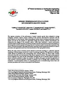
2.3 Adopted approaches This paper examines three approaches for assessment of the seismic performance in the context outlined above as follows: (1) Pseudo-static analysis within a deterministic approach incorporating parametric evaluation (DAp) (2) Seismic effective stress analysis using a single scenario (DA) (3) Probabilistic approach based on the so-called PEER framework (Cornell and Krawinkler, 2000) using the seismic effective stress analysis as a computational method (PA) These assessment approaches can be applied to various earth structures and soil-structure systems, but here they are applied to the assessment of seismic performance of pile foundations in liquefiable soils. 2.4 Case study The Fitzgerald Avenue Bridge over the Avon River in Christchurch, New Zealand, will be used as a case study. It is a small-span twin-bridge that has been identified as an important lifeline for post-disaster emergency services. Hence, the bridge has to remain operational in the event of a strong earthquake. To this goal, a structural retrofit has been considered involving widening of the bridge and strengthening of the foundation with new large diameter piles. A cross section at the mid span of one of the bridges is shown in Figure 3 where both existing piles and new piles are shown.
Figure 4 depicts the SPT blow count and soil profile at the northeast corner of the bridge. This soil profile was adopted in the pseudo-static analyses. The soil deposit consists of relatively loose liquefiable sandy soils with a thickness of about 15 m overlying a denser sand layer. The sand layers have low fines content predominantly in the range between 3% and 15% by weight. Detailed SPT and CPT investigations revealed a large spatial variability of the penetration resistance at the site. Hence, a rigorous investigation of the seismic response of the bridge and its foundation would require consideration of 3-D effects and spatial variability of soils. These complexities are beyond the scope of this paper, however, and rather a simplified scenario will be 0 Sandy SILT N=12 Sandy GRAVEL
N=7
5 Depth (m)
while the probabilistic approach (PA) offers the most rigorous treatment of uncertainties and quantifies their effects on the computed seismic response.
10
N=14 SAND
15
Silty SAND Silty N=15 SAND
Assumed
20 25 0
N=8
N=30 SAND 20 40 60 80 SPT blow count, N
Liquefieable soil
Figure 4. SPT blow count and soil profile at the north-east abutment
considered herein with the principal objective being to examine the response of the pile foundation shown in Figure 3. Here, we will focus on the cyclic response of the foundation during the intense ground shaking; effects of lateral spreading are beyond the scope of this study. 3 PSEUDO-STATIC ANALYSIS 3.1 Objectives As a practical approach, the pseudo-static analysis should be relatively simple, based on conventional geotechnical data and applicable without requiring significant computational resources. In addition, in order to satisfy the PBEE objectives in the seismic performance assessment, the pseudo-static analysis of piles should: - Capture the relevant deformational mechanism for piles in liquefying soils - Permit estimation of the inelastic response and damage to piles, and - Address the uncertainties associated with seismic behaviour of piles in liquefying soils. Not all available methods for simplified analysis satisfy these requirements. In particular, in the current practice the treatment of uncertainties in the simplified analysis is often inadequate; commonly, the uncertainties are either ignored or poorly addressed in the analysis. In what follows, a recently developed method for pseudo-static analysis of piles in liquefying soils (Cubrinovski and Ishihara, 2004; Cubrinovski et al., 2009) is used to assess the seis-
a) Cross section
mic performance of the new piles of Fitzgerald Bridge. Key features of the simplified analysis and effects of uncertainties on the pile response are discussed. 3.2 Computational model and input parameters Although in principle the pseudo-static analysis could be applied to a pile group, typically it is applied to a single-pile model. This is consistent with the overall philosophy for a gross simplification adopted in this approach. A typical beam-spring model representing the soil-pile system in the simplified pseudo-static analysis is shown in Figure 5. The model can easily incorporate a stratified soil profile (multi-layer deposit) with different thickness of liquefied layers and a crust of non-liquefiable soil at the ground surface. Since one of the key requirements of the analysis is to estimate the inelastic deformation and damage to the pile, in the proposed model simple but non-linear load-deformation relationships are adopted for the soil-pile system. The soil is represented by bilinear springs in which degraded stiffness and strength of the soil are used to account for effects of nonlinear behaviour and liquefaction. The pile is modelled using a series of beam elements with a tri-linear moment-curvature relationship. Parameters of the model are illustrated in Figure 5 for a typical three-layer configuration in which a liquefied layer is sandwiched between a surface layer and a base layer of non-liquefiable soils. All model parameters are based on conventional geotechnical data (SPT blow count) and concepts
b) Numerical scheme
UG HHC Non-liquefied
UP p
Lateral load, F
kC
crust layer
M
HL
δ
U
Y
Free field ground displacement
pC-max
C
φ
Liquefied layers
p
pL-max
β kL
δ
Deformed pile
Pile
HB Non-liquefied base layer
p kB pB-max
Soil spring
δ
Figure 5. Beam-spring model for pseudo-static analysis of piles (model parameters and characterization of nonlinear behav-
3.3 Uncertainties in the parameters of the model The pseudo-static analysis aims at estimating the maximum response of the pile under the assumption that dynamic loads can be idealized as static actions. Since behaviour of piles in liquefying soils is extremely complex involving very large and rapid changes in soil stiffness, strength and lateral loads on the pile, the key question in the implementation of the pseudo-static analysis is how to select appropriate values for the soil stiffness, strength and lateral loads on the pile for the equivalent static analysis. In other words, what are the appropriate values for β, pL-max, UG and F in the model shown in Figure 5? The following discussion illustrates that this choice is not straightforward and that all these parameters may vary within a wide range of values. In the adopted model, effects of liquefaction on stiffness of the soil are taken into account through the degradation parameter β. Observations from fullsize experiments and back-calculations from case histories indicate that for cyclic liquefaction (excluding lateral spreading), β typically takes values in the range between 1/10 and 1/50 (Cubrinovski et al., 2006). Similar uncertainty exists regarding the ultimate pressure from the liquefied soil on the pile or the value of pL-max in the model. The ultimate lateral pressure pL-max can be approximated using the residual strength of liquefied soils (Sr) as pL-max = αLSr. There are significant uncertainties regarding both αL and Sr values. The latter is illustrated by the scatter of the data in the empirical correlation between the residual strength of liquefied soils and normalized SPT blow count (N1)60cs (Seed and Harder, 1991) shown in Figure 6. For example, for a normalized equivalent-sand blow count of (N1)60cs = 10, the residual strength varies approximately between 5 kPa and 25 kPa. The selection of appropriate equivalent static loads is probably the most difficult task in the pseudo-static analysis. This is because both input loads in the pseudo-static analysis (UG and F) are in effect estimates for the seismic responses of the free field ground and soil-pile-structure system respectively. The magnitude of lateral ground displacement UG can be estimated using simple empirical models based on SPT charts such as that proposed by Tokimatsu and Asaka (1998). Using this method, a value
Residual shear strength, Sr (kPa)
(subgrade reaction coefficient, Rankine passive pressure). In the model, two equivalent static loads are applied to the pile: a lateral force at the pile-head (F) representing the inertial load due to vibration of the superstructure, and a horizontal ground displacement (UG) applied at the free end of the soil springs (Fig. 5b) representing the kinematic load on the pile due to lateral movement of the free field soils.
60 50
p
S r-UB S
r-LB
40
δ
30
Range of data presented by Seed & Harder (1991)
S
r-UB
Upper bound
Used for RM
20 10
S
r-LB
Lower bound
00
5 10 15 20 Equivalent clean sand SPT blow count, (N ) 1 60cs
Figure 6. Residual shear strength of liquefied sandy soils (after Seed and Harder, 1991)
of UG = 0.36 m was estimated for the maximum cyclic ground displacement at Fitzgerald Bridge site. Note that since UG is an estimate for the free field response at the site, it is reasonable to expect a considerable variation in the value of UG around the above estimate based on an empirical model. As mentioned earlier, the objective of the pseudostatic analysis is to estimate the peak response of the pile that will occur during an earthquake. The peak loads on the pile due to ground movement and vibration of the superstructure do not necessarily occur at the same time, and hence, there is no clear and simple strategy how to combine these loads in a static analysis. Recently, Boulanger et al. (2007) suggested that the maximum ground displacement should be combined with an inertial load from the vibration of the superstructure proportional to the peak ground acceleration amax using the following expression: F = Icmsamax. Here, ms is the mass of the superstructure whereas Ic is a factor that depends on the period of the earthquake motion and practically provides a rule for combining the kinematic (UG) and inertial (F) loads on the pile. Again, a wide range of values have been suggested for this parameter: Ic = 0.4, 0.6 and 0.8 for a short, medium and long period ground motions respectively (Boulanger et al., 2007). 3.4 Computed response for a reference model (RM) Based on the procedures outlined above, a so-called reference model (RM) was defined for the pile foundation of Fitzgerald Bridge. RM is a single pile model for the new piles (1.5m in diameter) in which a ‘mid range’ values were adopted for the parameters of the model, as summarized in Table 1. Here, the Sr values of 14 and 36 were derived using the broken line in Figure 6 and normalized blow counts of (N1)60cs = 10 and 15 respectively, for the liquefiable layers. The pile was subjected to a free field ground displacement with a peak value at the ground
Sr-LB
Variation in pile displacement due to properties of liquefied soils
Variation in bending moment due to properties of liquefied soils
Sr-LB
S r-UB
0
S r-UB
0
(b)
(a)
Mc
5
5
My Mu
10
Pile displacement
15
Applied free field ground displacement
Depth (m)
Depth (m)
RM 10 My 15
20
20
25
25
0 0.1 0.2 0.3 0.4 0.5 Horizontal displacement (m)
RM Mu
-10
Mc
-5
0
5
10
Bending moment, MPH (MN-m)
Figure 7. Effects of properties of liquefied soils on the pile response computed in the pseudo-static analysis: (a) pile displacements; (b) bending moments
surface of UG = 0.36m, indicated in Figure 7a, and a lateral load at the pile head corresponding to a peak ground acceleration of amax = 0.4g and an inertial coefficient of Ic = 0.6. The computed pile displacement and bending moment for the reference model (RM) are shown with solid lines in Figures 7a and 7b respectively. A pile head displacement of 0.21m and a peak bending moment at the pile head of 9.6 MN-m were computed. The bending moment exceeded the yield level both at the pile head and at the interface between the liquefied layer and underlying base layer. Table 1. Characteristic values of model parameters _______________________________________________ RM Range of values Parameter _____________ LB* UB** _______________________________________________ β 1/20 1/50 - 1/10 Sr (N1=10) (kPa) 14 6 - 22 Sr (N1=15) (kPa) 36 24 - 48 Ic 0.6 0.4 - 0.8 U (m) 0.36 0.29 - 0.43 G _______________________________________________ * Lower Bound (minimum value) ** Upper Bound (maximum value)
3.5 Effects of uncertainties on the pile response To examine the effects of uncertainties associated with the liquefied soil and lateral loads on the pile, parametric analyses were carried out in which the above parameters were varied within the relevant range of values listed in Table 1. For example, an analysis was conducted in which RM values were used for all parameters except for the stiffness degradation (β) and residual strength (Sr) of the lique-
fied soil, for which instead the lower bound or minimum values of β = 1/50, Sr = 6 kPa (N1 = 10) and Sr = 24 kPa (N1 = 15) were used. Similarly, another analysis was conducted in which the upper bound or maximum values of β = 1/10, Sr = 22 kPa (N1 = 10) and Sr = 48 kPa (N1 = 15) were used in conjunction with the RM values for all other parameters. Results of these two analyses are shown in Figure 7 indicating significant effects of the spring properties for the liquefied soil on the pile response. Figure 8 shows results from a similar pair of analyses in which the value for the applied ground displacement was either decreased (UG = 0.29m) or increased (UG = 0.43m) for 20% with respect to the RM displacement of 0.36m. Again, a large difference in the pile response is seen resulting from a relatively small variation in the ground displacement applied to the pile. Results of the parametric analyses are summarized in Table 2 and are depicted in tornado charts for the pile head displacement and bending moment (at the pile head) respectively in Figures 9a and 9b. The response of the reference model (RM) is also indicated in these plots for comparison purpose. The results clearly indicate that the pile response is significantly affected by the adopted values for stiffness and strength of the liquefied soil, and to a lesser extent by the adopted values for loads, UG and F (due to variation of Ic between 0.4 and 0.8). Note that the size of these effects will change with the properties of the soil-pile system (especially with the stiffness of the pile relative to that of the soil), degree of yielding in the soil and pile, and the size of lateral loads from a non-liquefied crust at the ground surface.
Variation in pile displacement due to applied U
Variation in bending moment due to applied U
G
UG = 0.29m 0
G
0
(a)
(b)
10 15
Applied free field ground displacement
Mc
5
RM (UG = 0.36m) Depth (m)
Depth (m)
5
UG = 0.43m
UG = 0.29m
UG = 0.43m
10 My
RM (UG = 0.36m)
15
20
20
25
25
0 0.1 0.2 0.3 0.4 0.5 Horizontal displacement (m)
My Mu
Mu
-10
Mc
-5
0
5
Bending moment, M
PH
10 (MN-m)
Figure 8. Effects of applied lateral ground displacement on the pile response computed in the pseudo-static analysis: (a) pile displacements; (b) bending moments
(a) Table 2. Results of parametric analyses ___________________________________________ Model Pile response _____________ UPH* MPH** ___________________________________________ RM with Sr-LB and β2-LB 0.10 7.8 RM with UG = 0.29m 0.16 8.9 RM with Is-LB = 0.4 0.18 8.9 RM 0.21 9.5 RM with UG = 0.43m 0.25 9.9 RM with Is-UB = 0.8 0.23 10.0 RM with Sr-UB and β2-UB 0.27 10.3 ___________________________________________ * Pile-head displacement ** Bending moment at pile head
3.6 Discussion The above results clearly illustrate a high sensitivity of the pile response on the parameters of the simplified model. This sensitivity is not specific to the adopted approach in this study, but rather is a common feature of simplified methods of analysis. It simply reflects the significant uncertainties associated with the complex phenomena considered and their gross simplification in the pseudo-static method of analysis. The results also clearly emphasize the need for a parametric evaluation of the seismic response when using simplified methods of analysis. In terms of the previously introduced assessment approaches, a deterministic approach including parametric analyses (DAP) would be required when using simplified methods of analysis for seismic performance assessment. In the current practice, various methods for simplified (pseudo-static) analysis are used. These methods are similar in principle however they all
(b) S ,β
S ,β
r
r
U
G
LB
UB
F(Is)
U
G
LB
UB
F(Is) RM
RM 0.1 0.2 0.3 Pile head displacement, U (m) PH
7
8 9 10 11 Bending moment, MH (MNm)
Figure 9. Tornado charts depicting pile response computed in parametric pseudo-static analyses: (a) pile-head displacement; (b) bending moment at pile head
have distinct modelling features and use different load-deformation relationships, geotechnical data and empirical correlations. For this reason, they all require an independent process of ‘calibration’ in which model parameters will be rigorously examined and their relevant range of values identified. Note that this calibration is both model-specific and problem-specific. For example, the pseudo-static analysis method presented herein when applied to the assessment of piles subjected to lateral spreading will need different set of reference values for the model parameters, e.g. magnitude of UG, load combination rule for UG and F, and stiffness degradation factor β.
4 SEISMIC EFFECTIVE STRESS ANALYSIS 4.1 Implementation steps Unlike the simplified analysis procedure where the response of the pile is evaluated using a beam-spring model and equivalent static loads as input, the seismic effective stress analysis incorporates the soil, foundation and superstructure in a single model and uses an acceleration time history as a base excitation for this model. This analysis aims at a very detailed modelling of the ground response and soil-structure system in a rigorous dynamic analysis. The seismic effective stress analysis is difficult to implement in practice because it requires significant computational resources and specialists knowledge from the user. In concept, the effective stress analysis could be considered as the opposite approach to that of the practical pseudo-static analysis. The implementation of the effective stress analysis generally involves three steps (Fig. 10): (1) Determination of the parameters of the constitutive model (2) Definition of the numerical model (3) Dynamic analysis and interpretation of results In the first step, parameters of the constitutive model for the soil are determined using results from laboratory tests on soil samples and data from in-situ investigations. The required types of laboratory tests are model-specific and are generally used for determination of stress-strain relationships and effects of excess pore pressures on the soil response (liquefaction tests). Whereas most of the constitutive model parameters can be directly evaluated from data obtained from laboratory tests and in-situ investigations, some parameters are determined through a calibration process in which best-fit values for the parameters are identified in simulations of laboratory tests (so-called element test simulations). In the second step, the numerical model is defined by selecting appropriate element types, dimensions of the model, mesh size, boundary conditions and initial stress state. The last two requirements often receive less attention, even though they have pivotal influence on the performance of the constitutive model and numerical analysis. Namely, one of the key advantages of the advanced numerical analysis is that no postulated failure and deformation modes are required, as these are predicted by the analysis itself. In this context, the selection of apSTEP 1
Determination of parameters of the constitutive model - Laboratory tests - In-situ investigations - Element test simulations
propriate boundary conditions along end-boundaries and soil-foundation-structure interfaces are critically important in order to allow unconstrained response and development of relevant deformation modes. Similarly, stress-strain behaviour of soils and liquefaction resistance are strongly affected by the initial stress state of the soil, and therefore, an initial stress analysis is required to determine gravity-induced stresses in all elements of the model resembling those in the field. In the final step, an acceleration time history (ground motion) is selected which is used as a base excitation for the model. Considering the geometry of the problem and anticipated behaviour, numerical parameters such as computational time increment, integration scheme and numerical damping are adopted, and the dynamic effective stress analysis is then executed. The analysis is quite demanding on the user in all steps including the final stages of post-processing and interpretation of results since it requires an in-depth understanding of the phenomena considered, constitutive model used and particular numerical procedures adopted in the analysis. Benchmarking exercises imply that these rigorous requirements are not always satisfied in the profession even when dealing with static problems (Potts, 2003). In cases when the analysis is used for a rigorous assessment of the seismic performance of important structures, high-quality geotechnical data from field investigations and laboratory tests are needed in order to model the particular deformational characteristics (stress-strain relationships) of the soils in questions. Such data are rarely available, however, and this has been often used as an excuse to avoid using the seismic effective stress analysis in geotechnical practice. However, even when conventional data is used as input, this analysis still provides an important and unique contribution in the seismic performance assessment of earth structures and soilfoundation-structure systems, as illustrated below. 4.2 Numerical model The 2-D finite element model adopted for the effective stress analysis of the pile foundation of Fitzgerald Bridge is shown in Figure 11. The model includes the soil, pile foundation (both existing piles and new piles) and the superstructure. Four-node
STEP 2
Definition of numerical model - Element types and FE mesh - Boundary conditions - Modelling of interfaces - Initial stress state
Figure 10. Key steps in the implementation of seismic effective stress analysis
STEP 3
Dynamic analysis - Ground motion (input) - Numerical parameters - Postprocessing - Interpretation of results
Bridge superstructure Elastic solid elements with appropriate tributary mass
Piles Non-linear beam elements with hyperbolic M-φ relationship
Soil elements (Two-phase solid elements; elasti-plastic constitutive model for sand) Figure 11. Numerical model used in the seismic effective stress analysis of Fitzgerald Bridge
solid elements were employed for modelling the soil and bridge superstructure while beam elements were used for the piles and pile cap. Lateral boundaries of the model were tied to share identical displacements in order to simulate a free field ground motion near the boundaries. Along the soil-pile interface, the piles and the adjacent soil were connected at the nodes and were forced to share identical horizontal displacements. The footing, bridge deck and pier were all modelled as linear elastic materials with an appropriate tributary mass to simulate inertial effects from the superstructure. Nonlinear behaviour of the piles was modelled with a hyperbolic moment-curvature (M-φ) relationship while the soil was modelled using an elastic-plastic constitutive model developed specifically for modelling sand behaviour and liquefaction problems (Cubrinovski and Ishihara, 1998a; 1998b). Details of the constitutive law and numerical procedures will not be discussed herein, but rather modelling of the liquefaction resistance based on conventional geotechnical data will be demonstrated. The model shown in Figure 11 was subjected to an earthquake excitation with similar general attributes (magnitude, distance and PGA) to those relevant for the seismic hazard of Christchurch. An acceleration record obtained during the 1995 Kobe earthquake (M=7.2) was scaled to a peak acceleration of 0.4g and used as a base input motion. Needless to say, the adopted input motion is neither representative of the source mechanism nor path effects specific to Canterbury, but rather it was considered a relevant excitation typical for the size of the earthquake event considered in the analysis. 4.3 Modelling of liquefaction resistance For a rigorous determination of parameters of the employed constitutive model, about 15 to 20 laboratory tests are required including monotonic and cyclic, drained and undrained shear tests. In the absence of laboratory tests for the soils at the Fitzgerald Bridge site, the constitutive model parameters were determined by largely adopting the parameters of Toyoura sand (Cubrinovski and Ishi-
hara, 1998a) and modifying the dilatancy parameters as described below. Borelogs, penetration resistance data from CPTs and SPTs and conventional physical property tests were the only geotechnical data available for the soils at Fitzgerald Bridge site. A rudimentary modelling of stress-strain behaviour of soils considering liquefaction would require knowledge or assumption of the initial stiffness of the soil, strength of the soil and liquefaction resistance. Since none of these were directly available for the soils at this site they were inferred based on the measured penetration resistance. The liquefaction resistance was determined using the conventional procedure for liquefaction evaluation based on empirical SPT charts (Youd et al., 2001). After an appropriate correction for the fines content and the magnitude of the earthquake (using magnitude scaling factor), these charts provided the cyclic stress ratios required to cause liquefaction in 15 cycles, which are shown by the solid symbols in Figure 12. Using these values as a target liquefaction resistance, the dilatancy parameters of the model were determined and the liquefaction resistance was simulated for the two layers, as indicated with the lines in Figure 12. These two lines represent the simulated liquefaction resistance curves for the soils with N1 = 10 and N1 = 15 respectively. To illustrate better this process, results of element test simulations for the sand with N1 = 10 are shown in Figure 13 where effective stress paths and stress-strain curves are shown for three different cyclic stress ratios of 0.12, 0.18 and 0.30 respectively. The number of cycles required to cause liquefaction in these simulations and the corresponding stress ratios are indicated with open symbols in Figure 12, depicting the simulated liquefaction resistance. Thus, only conventional data were used for determination of model parameters. While this choice of material parameters practically eliminates the possibility for a rigorous quantification of the seismic response of the soil-pile-structure system, one may argue that the parameters of the model defined as above are at least as consistent and credible as those used in a conventional liquefaction evaluation.
vo
Cyclic stress ratio, τ/σ '
0.5 0.4
Based on conventional liquefaction evaluation N = 15
0.3
1
C
0.2 N = 10 1
0.1 0
B A
1
10 Number of cycles, N
100
c
30 CSR=0.12 20 10 0 -10 -20 40 cycles to liquefaction -30 0 20 40 60 80 100 Mean effective stress , p' (kPa)
Shear stress, τ (kPa)
30 CSR=0.18 20 10 0 -10 -20 10 cycles to liquefaction -30 0 20 40 60 80 100 Mean effective stress , p' (kPa)
Shear stress, τ (kPa)
30 CSR=0.30 2 cycles to 20 liquefaction 10 0 -10 -20 -30 0 20 40 60 80 100 Mean effective stress , p' (kPa)
Shear stress, τ (kPa)
Shear stress, τ (kPa)
Shear stress, τ (kPa)
Shear stress, τ (kPa)
Figure 12. Liquefaction resistance curves adopted in the seismic effective stress analysis (curves represent model simulations)
30 20 10 0 -10 -20 -30
CSR=0.12 Point A: CSR=0.12 40 cycles
-4
30 20 10 0 -10 -20 -30
2 (%)
4
CSR=0.18 Point B: CSR=0.18 10 cycles
-4
30 20 10 0 -10 -20 -30
-2 0 Shear strain, γ
-2 0 Shear strain, γ
2 (%)
4
CSR=0.30 Point C: CSR=0.30 2 cycles
-4
-2 0 2 4 Shear strain, γ (%)
Figure 13. Effective stress paths and stress-strain curves obtained in element test simulations for the soil layer with N1 = 10
4.4 Computed ground response Figure 14a shows time histories of excess pore water pressure computed at two depths corresponding to the mid depth of layers with N1 = 10 and N1 = 15 (z = 13.2m and 7.0m respectively). In the weaker layer, the pore water pressure builds-up rapidly in only one or two stress cycles until a complete liquefaction of this layer was reached at approximately 15 seconds. In the denser layer (N1 = 15), the pore water pressure build up is slower and affected by the liquefaction in the underlying looser layer. The latter is apparent in the reduced rate of pore pressure increase after 15 seconds on the time scale. Clearly, the liquefaction of the loose layer at greater depth produced “base-
isolation” effects and curtailed the development of liquefaction in the overlying denser layer. Figure 14b further illustrates the development of the excess pore water pressure throughout the depth of the deposit with time. Note that part of the steady build up of the pore pressure in the upper layer (N1 = 15) is caused by “progressive liquefaction” or upward flow of water from the underlying liquefied layer. Needless to say, the pore pressure characteristics outlined in Figure 14 will be reflected in the development of transient deformation and permanent displacements of the ground. The seismic effective stress analysis can simulate these complex features of the ground response and their effects on structures.
vo
Pore water pressure ratio (u/σ' )
1.2
z = 13.2m
1
Pore water pressure ratio (u/σ' ) vo 0 0.25 0.5 0.75 1 0
(a)
t=40s
0.8
10
5
0.6
15
z = 7.0m Depth (m)
0.4 0.2 0
t=25s
10
t=15s
15 (b)
20
0
10
20
30 40 Time (s)
50
N =10 1
-0.2 -0.4
End
60 25
Figure 14. Computed excess pore water pressure in the free field soil: (a) time histories at mid-depths of layers with N1 = 10 and N1 = 15; (b) distribution of excess pore water pressures throughout the depth of the deposit and time
4.5 Computed pile response The computed time history of horizontal displacement of the pile is shown in Figure 15a together with the corresponding displacement of the ground in the free field. The peak pile displacement reached about 0.18m at the pile head, which is significantly smaller than the peak free field displacement at the ground surface of 0.30m indicating relatively stiff pile behaviour (the pile is resisting the ground movement). The response shown in Figure 15a indicates that the peak displacements of the pile and free field soil occurred at different times, at approximately 19 seconds and 32 seconds, respectively. The peak bending moment of the pile was at-
tained at the pile head (MH) with values slightly below the yield level (Figure 15b). This time history indicates not only the peak level of the response but also the number of significant peaks exceeding cracking level which in turn provides additional information on the damage to the pile. Similar level of detail is available for other components of the numerical model including the foundation soil, old and new piles, and response of the superstructure. 4.6 Discussion As illustrated in the above application, the seismic effective stress analysis allows realistic and detailed
Horizontal displacement (m)
0.4
(a)
0.2
Free-field displacement (at ground surface)
0 -0.2 -0.4
Pile-head displacment 0
10
20
30
40
50
60
M
(b) (MN-m)
Bending moment at pile head, M
PH
10 5
Mc
0 -5 -10 0
y
Mc M 10
y
20
30
40
50
60
Time (s)
Figure 15. Computed response of the pile in seismic effective stress analysis: (a) horizontal displacement at pile head; (b) bending moment at pile head
simulation of the seismic response of geotechnical structures induced by strong earthquakes. Effects of soil-structure interaction are easily included in the analysis, in which sophisticated nonlinear models can be used both for soils and for structural members. The analysis permits a rigorous assessment of the seismic performance of the soil-structure system as a whole and each of its components. Effects of excess pore water pressure are often a key factor in the seismic response of ground and earth structures. Hence, the ability of this analysis to capture details of pore pressure build-up, development of liquefaction and consequent loss of strength and stiffness in the soil is of great value. The method simulates the most salient features of seismic behaviour of soils including peculiar effects from individual layers and cross interaction amongst them such as “base-isolation effects” or progressive liquefaction due to upward flow of water. Because of its complexity and high-demands on the user, the seismic effective stress analysis is typically applied in a deterministic fashion using a single scenario (DA) or input ground motion. However, this analysis also provides an excellent tool for assessment of alternative design solutions, effectiveness of structural strengthening and soil remediation (countermeasures against liquefaction) on a comparative basis by quantifying their effects on the ground deformation, structural response and reduction (control) of damage.
employs an integrated probabilistic treatment of all uncertainties that apply to the prediction of ground motion and evaluation of system response and associated damage (uncertainties associated with characteristics of ground motion, material properties, modelling approximations, seismic response and associated physical damage for a given response measure). Hence, it provides an alternative and more rigorous way for assessment of seismic performance of engineering structures. Recently, attempts have been made to expand the application of this approach to geotechnical problems (Kramer, 2008; Ledezma and Bray, 2007; Bradley at. al., 2008). Details of the probabilistic PBEE assessment are beyond the scope of this paper, and instead key features and implementation of this procedure will be outlined in the following using the case study considered. 5.2 Analysis procedure Christchurch is located in a region of relatively high seismicity and Fitzgerald Bridge is expected to be excited by a number of earthquakes during its lifespan. Considering all possible earthquake scenarios, the response of the bridge and its pile foundation needs to be evaluated for earthquakes with different intensities ranging from very weak and frequent earthquakes to very strong but rare earthquakes. Characteristics of ground motions caused by these earthquakes are very difficult to predict because of the complex and poorly understood source mechanism, propagation paths of seismic waves and surface-soil effects. In order to account for these uncertainties in the ground motion characteristics, the following procedure was adopted. A suite of 40 ground motions recorded during strong earthquakes was first selected, as indicated in Figure 16a. Next, each of these records was scaled to ten different peak amplitude levels, i.e. peak
5 PROBABILISTIC APPROACH 5.1 Background A probabilistic approach (PEER framework) for Performance-Based Earthquake Engineering (PBEE) has been recently developed for a robust assessment of seismic performance of structures (Cornell and Krawinkler, 2000; Krawinkler 1999). This approach
(a) 40 Earthquake Records EQ1: Northridge 1994 EQ2: Imperial Valley 1979
(b) 400 Ground Motions GM1: EQ1, a
= 0.1 g
GM2: EQ1, a
= 0.2 g
max max
(c) 400 Time History Analyses
EQ40: Kobe 1995 GM10: EQ1, a
= 1.0 g
GM11: EQ2, a
= 0.1 g
max max
GM399: EQ40, a
= 0.9 g
GM400: EQ40, a
= 1.0 g
max max
Input motion
Figure 16. Schematic illustration of multiple effective stress analyses used in the probabilistic approach
0.7
(a)
0.6 0.5 0.4 0.3 0.2 0.1 0 0
0.25 0.5 0.75 1 Peak ground acceleration, a
max
1.25 (g)
Peak pile-head displacment, UPH (m)
Peak pile-head displacment, UPH (m)
0.8
0.8 0.7
(b)
0.6 0.5 0.4 0.3 0.2 0.1 0 0 200 400 600 800 Velocity spetrum intensity, VSI (cm/s)
Figure 17. Computed pile-head displacements (UPH) in 400 effective stress analyses: (a) correlation between (UPH) and amax of input motion; (b) correlation between (UPH) and velocity spectrum intensity (VSI) of input motion
ground accelerations of amax = 0.1, 0.2, 0.3, 0.4, 0.5, 0.6, 0.7, 0.8, 0.9 and 1.0 g. Thus, 400 different ground motions were generated in this way, as indicated in Figure 16b, having very different amplitudes, frequency content and duration. Using each of these time histories as a base input motion, 400 effective stress analyses were conducted using the model shown in Figure 11 and procedures outlined earlier, as schematically depicted in Figure 16c. 5.3 Computed response The next challenge to overcome is how to present results from 400 time history analyses in a meaningful way. Obviously, some relaxation in the rigorous treatment of time histories and evaluation of the response is needed here. In the probabilistic PBEE approach, this is achieved through the following reasoning: (1) First, the object of assessment is identified. Thus, instead of examining the entire soil-pilestructure system, for example, the attention is focused on the response of the pile. (2) Next, a representative measure for the response of the pile is identified, i.e. a parameter that describes and quantifies the pile response efficiently (“Engineering Demand Parameter”, EDP in the PBEE terminology). Hence, instead of using the entire time history of the pile response, the peak value of the response parameter (EDP) is used as a measure for the size of the response. (3) Similarly, a single parameter is used to describe the input motion or measure the intensity of the ground motion (“Intensity Measure”, IM). (4) Finally, the results of the analyses are presented by correlating the parameter represent-
ing the size of the response (EDP) with the intensity of the ground motion (IM). For example, one way of presenting the results from the 400 analyses with respect to the pile response for Fitzgerald Bridge is shown in Figure 17a where the peak displacement at the pile head (UPH) computed in the analysis is plotted against the peak acceleration of the input motion (amax). Here, UPH represents a measure for the size of the pile response (EDP) while amax is a measure for the intensity of the ground motion (IM). Each open symbol in Figure 17a represents the result (peak response of the pile) from one of the 400 seismic effective stress analyses while the solid line is an approximation of the trend from a regression analysis. The scatter of the data in Figure 17a is quite large indicating a significant uncertainty in the prediction of the peak response of the pile based on the peak acceleration of the ground motion (input PGA). Clearly one issue in this approach is the need to identify an efficient intensity measure that reduces the uncertainty and hence improves the predictability of the pile response. However, there is no wideranging intensity measure that is appropriate for all problems but rather the intensity measure is problem-dependent and is affected by the particular deformational mechanism and features of the phenomena considered. Based on detailed numerical studies, Bradley et al. (2008) have identified that velocitybased intensity measures correlate the best with the seismic response of piles, and that in particular the velocity spectrum intensity (VSI) is the most efficient intensity measure for piles. This is illustrated in Figure 17b where the same results for UPH from the 400 analyses shown in Figure 17a are re-plotted using VSI as the intensity measure for the employed input motions. The improved efficiency and predictability of the pile response is evident in the reduced
0
10
-1
10
-2
10
-3
10
-4
10
-5
10
-6
(a) DBE (1/475yr)
0
MCE (1/2475yr)
0.5 1 Peak ground acceleration, a
max
1.5 (g)
Mean annual rate of exceedance
Mean annual rate of exceedance
10
10
0
10
-1
10
-2
10
-3
10
-4
10
-5
10
-6
(b) Existing foundation Strengthened foundation
UPH at yielding
0 0.2 0.4 0.6 0.8 1 Peak pile-head displacement, U (m) PH
Figure 18. Probabilistic assessment of seismic performance of pile foundation: (a) seismic hazard curve for Christchurch; (b) Demand hazard curve for piles of Fitzgerald Bridge
uncertainty as depicted by the smaller dispersion of the data. The plots shown in Figure 17 provide means for estimating the peak response of the piles of Fitzgerald Bridge for all levels of earthquake excitation, from elastic response to failure. 5.4 Assessment of seismic performance: Demand hazard curve A conventional output from Probabilistic Seismic Hazard Analysis (PSHA) is the so-called seismic hazard curve which expresses the aggregate seismic hazard at a given site by considering all relevant earthquake sources contributing to the hazard. A seismic hazard curve for Christchurch (Stirling et al., 2001) is shown in Figure 18a where a relationship between the peak ground acceleration (amax) and mean annual rate of exceedance of a given amax is shown. For example, this hazard curve indicates that an earthquake event generating an amax = 0.28g in Christchurch has a recurrence interval or return period of 475 years (or 10% probability of exceedance in 50 years). By combining the seismic hazard curve expressed in terms of amax (Fig. 18a) and the correlation between the peak pile response (UPH) and amax established from the results of the effective stress analyses (Fig. 17a), a so-called “Demand Hazard Curve” was produced, shown in Figure 18b for the existing and new piles respectively. In this way, the probability for exceedance of a certain level of peak pile displacement in any given year (annual rate of exceedance) could be estimated for the piles of Fitzgerald Bridge. A unique feature of the demand hazard curve is that it provides an assessment of the seismic performance of the pile foundation by considering all earthquake scenarios for the site in question and associated uncertainties in the characterization of the ground motion.
In the above interpretation, the peak pile displacement was adopted as a measure for the size of the pile response because it is a good indicator of the peak deformation and damage to the pile (Bradley et al., 2008). Thus, UPH can be converted to a parameter directly correlating with the damage to the pile (the peak curvature of the pile), and then the demand hazard curve can be easily expressed in terms of a damage measure, thus providing likelihood of characteristic damage levels for the pile (cracking, yielding, failure). Furthermore, the physical damage of the pile foundation will lead to losses, and hence, the demand hazard curve can be also used to quantify the seismic performance in terms of economic measures (dollars). This in turn will provide an economic basis for decisions on seismic design, repair and retrofit, and will facilitate communication of the design outside the profession. Clearly, the probabilistic assessment provides alternative measures of the seismic performance of the pile while rigorously accounting for the uncertainties associated with the seismic hazard and phenomena considered. This approach can be applied to seismic performance assessment of any other component of the soil-pilestructure system and to the bridge as a whole. Also, other sources of uncertainty such as those related to modelling, soil and site characterization can be easily incorporated in the analysis and their effects on the response can be quantified. 6 SUMMARY AND CONCLUSIONS Three different approaches for assessment of the seismic performance of earth structures and soilstructure systems have been presented. These approaches use different models, analysis procedures and are of vastly different complexity. All are consistent with the performance-based design philoso-
phy according to which the seismic performance is assessed using deformational criteria and associated damage; however, they focus on different aspects and make different contribution in the assessment. Key features of the examined approaches and their specific contribution in the seismic performance assessment are summarized in Table 3. 6.1 Pseudo-static analysis The pseudo-static analysis is a practical approach based on conventional geotechnical data, engineering concepts and relatively simple computational models. It postulates a specific deformational mechanism and aims at estimating the peak response of the pile due to an earthquake under the assumption that dynamic loads can be represented as static actions. The method is easy to implement in practice and provides a suitable tool for evaluation of the seismic response of piles and associated damage to piles. This approach focuses on the pile itself (enhances foundation design) while it ignores the response of the system and other components of the system. In addition to the uncertainties associated with the complex seismic behaviour and ground motion, there are significant uncertainties related to modelling arising from unknown variables and inaccurate model form. These modelling uncertainties are very pronounced in the simplified analysis because of the significant approximations and gross simplification of the problem adopted in this approach. Thus, when using simplified methods of analysis in the assessment, it is critically important to address these uncertainties through systematic parametric studies. 6.2 Seismic effective stress analysis The seismic effective stress analysis aims at a very
realistic simulation of the seismic behaviour of earth structures and soil-structure systems. It incorporates sophisticated nonlinear models for the soil, foundation and structure in a rigorous dynamic analysis. The key contribution of this analysis is that it allows examining in detail the performance of the soilstructure system under a strong earthquake excitation. Even results from a single analysis (such as that presented herein) illustrate the benefit of a detailed soil-pile-structure analysis. The experience from recent strong earthquakes suggests that design concepts in which pile foundations are considered to remain within the elastic range of deformation during strong earthquakes are not economical. The PBEE philosophy also suggests accepting damage in seismic events, if this proves the most economic solution (Krawinkler, 1999). Hence, there is a need to consider inelastic deformation concurrently in both the superstructure and pile foundation, and to assess the performance both on a system level and at a component level (Gazetas and Mylonakis, 1998). Advanced numerical analyses provide this capability and methods based on the effective stress principle further permit consideration of important ground response features such as effects of excess pore pressures and liquefaction. Since this approach focuses on a detailed evaluation of the seismic response, it is not appropriate for parametric evaluation including large number of analyses. In this context, the selection of an appropriate input motion is problematic in cases when rigorous assessment and quantification of the seismic performance of important structures is needed. 6.3 Probabilistic approach The probabilistic approach offers a unique perspective in the assessment of seismic performance, first through a rigorous treatment of the single most im-
Table 3. Methods for seismic performance assessment of soil-structure systems: Key features and contributions in the assessment Method of assessment
Key features •
Pseudo-static analysis
•
Simple Conventional data and engineering concepts
Specific contributions in the assessment •
• •
Seismic effective stress analysis
Realistic simulation of ground response & seismic soilfoundation-structure interaction
•
•
• •
Probabilistic PBEE framework
•
Considers all earthquake scenarios Quantifies seismic risk
•
•
Shortcomings
Evaluates the response and damage level for the pile (parametric evaluation is needed) Enhances foundation design
•
Detailed assessment of seismic response of pile foundations including effects of liquefaction and SSI Integral assessment of inelastic behaviour of soilfoundation-structure systems Enhances communication of design concepts between geotechnical and structural engineers
•
Addresses uncertainties associated with ground motion characteristics on a site specific basis Provides engineering measures (response and damage) and economic measures (losses) of performance Enhances communication of design outside profession
•
Does not consider the response of the soil-foundationstructure system Ignores uncertainties in the ground motion
Ignores details of the seismic response
portant source of uncertainty in seismic studies, the ground motion, and then by providing alternative performance measures in the assessment, engineering and economic ones. It allows us to combine geotechnical and structural design aspects and to evaluate their effects on the performance of the entire system (soil-foundation-structure system) and each of its components. It is worth noting that in spite of the use of an effective stress analysis as a basic computational tool in the probabilistic approach employed herein, details of the response were not considered in the seismic performance assessment. 6.4 Future needs The examined approaches address different aspects in the assessment and, in essence, are complimentary in nature. It is envisioned that these approaches will be used in parallel in the future, and hence, they all require further development and improvement. The pseudo-static approach requires establishment of improved models depicting multiple deformational mechanisms and in particular more rigorous and systematic procedures for parametric evaluation of the seismic response. Methods based on seismic effective stress analysis require improvement in the simulation of large ground deformation and more emphasis on use of sophisticated nonlinear models for an integrated analysis of the soil-foundation-structure system. Finally, further development of the probabilistic approach is needed including efforts towards simplification of procedures and identification of representative response measures (EDPs) and ground motion measures (IMs) for various specific problems. All of these analysis procedures improve our understanding of complex seismic behaviour and enhance engineering judgement, which is probably one of the most significant contributions that one can expect from such an exercise. ACKNOWLEDGEMENTS The authors would like to acknowledge the financial support provided by the Earthquake Commission (EQC), New Zealand. REFERENCES Bradley, B., Cubrinovski, M. & Dhakal, R. 2008. Performance-based seismic response of pile foundations. ASCE Geotechnical Special Publication 181: 1-11. Boulanger, R. Chang, D., Brandenberg, S. & Armstrong, R. 2007. Seismic design of pile foundations for liquefaction effects. 4th Int. Conference on Earthquake Geotechnical Engineering-Invited Lectures, Ed. Pitilakis, 277-302. Bowen, H.J. & Cubrinovski, M. 2008. Effective stress analysis of piles in liquefiable soil: A case study of a bridge founda-
tion,” Bulletin of the NZ Society for Earthquake Engineering, 41(4): 247-262. Cornell, C.A. & Krawinkler, H 2000. Progress and challenges in seismic performance assessment. PEER Center News, 3(2):1-4. Cubrinovski, M. & Ishihara, K. 1998a. Modelling of sand behaviour based on state concept. Soils and Foundations 38(3): 115-127. Cubrinovski, M. & Ishihara, K. 1998b. State concept and modified elastoplasticity for sand modelling. Soils and Foundations 38(4): 213-225 Cubrinovski, M. & Ishihara, K. 2004. Simplified method for analysis of piles undergoing lateral spreading in liquefied soils. Soils and Foundations, 44(25): 119-133. Cubrinovski, M., Kokusho, T. & Ishihara, K. 2006. Interpretation from large-scale shake table tests on piles undergoing lateral spreading in liquefied soils. Soil Dynamics and Earthquake Engineering, 26: 275-286. Cubrinovski, M., Ishihara, K. & Poulos, H. 2009. Pseudostatic analysis of piles subjected to lateral spreading. Special Issue, Bulletin of NZ Society for Earthquake Engineering, 42(1): (in print). Gazetas G. & Mylonakis, G. 1998. Seismic soil-structure interaction: new evidence and emerging issues. ASCE Geotechnical Special Publication 75: 1119-1174. Kramer, S.L. 2008. Performance-Based Earthquake Engineering: opportunities and implications for geotechnical engineering practice. ASCE Geotechnical Special Publication 181: 1-32. Krawinkler, H. 1999. Challenges and progress in performancebased earthquake engineering. Int. seminar on seismic engineering for Tomorrow – In Honour of Professor Hiroshi Akiyama Tokyo, Japan, November 26, 1999:1-10. Ledezma, C. & Bray, J. 2007. Performance-based earthquake engineering design evaluation procedure for bridge foundations undergoing liquefaction-induced lateral spreading, PEER Report 2007: 1-136. Potts, D.M. 2003. Numerical analysis: a virtual dream or practical reality? The 42nd Rankine Lecture, Geotechnique 53(6): 535-573. Seed, R.B. & Harder, L.F. 1991. SPT-based analysis of cyclic pore pressure generation and undrained residual strength. H. Bolton Seed Memorial Symposium Proc., 2: 351-376. Stirling, M.W., Pettinga, J., Berryman, K.R. & Yetton, M. 2001. Probabilistic seismic hazard assessment of the Canterbury region, Bulletin of NZ Society for Earthquake Engineering 34: 318-334. Tokimatsu K. & Asaka Y. 1998. Effects of liquefactioninduced ground displacements on pile performance in the 1995 Hyogoken-Nambu earthquake. Special Issue of Soils and Foundations, September 1998: 163-177. Youd, T.L. & Idriss, I.M. 2001. Liquefaction resistance of soils: summary report from the 1996 NCEER and 1998 NCEER/NSF workshops on evaluation of liquefaction resistance of soils, Journal of Geotechnical and Geoenvironmental Engineering, 127(4): 297-313.