International Journal of Health Geographics
BioMed Central
Open Access
Research
Evaluation of the performance of tests for spatial randomness on prostate cancer data Virginia L Hinrichsen*1, Ann C Klassen2, Changhong Song3 and Martin Kulldorff1 Address: 1Department of Ambulatory Care and Prevention, Harvard Medical School and Harvard Pilgrim Health Care, Boston, MA 02215, USA, 2Department of Health, Behavior and Society, Johns Hopkins Bloomberg School of Public Health, Baltimore, MD 21205, USA and 3Department of Statistics, University of Connecticut, Storrs, CT 06269, USA Email: Virginia L Hinrichsen* -
[email protected]; Ann C Klassen -
[email protected]; Changhong Song -
[email protected]; Martin Kulldorff -
[email protected] * Corresponding author
Published: 3 July 2009 International Journal of Health Geographics 2009, 8:41
doi:10.1186/1476-072X-8-41
Received: 18 December 2008 Accepted: 3 July 2009
This article is available from: http://www.ij-healthgeographics.com/content/8/1/41 © 2009 Hinrichsen et al; licensee BioMed Central Ltd. This is an Open Access article distributed under the terms of the Creative Commons Attribution License (http://creativecommons.org/licenses/by/2.0), which permits unrestricted use, distribution, and reproduction in any medium, provided the original work is properly cited.
Abstract Background: Spatial global clustering tests can be used to evaluate the geographical distribution of health outcomes. The power of several of these tests has been evaluated and compared using simulated data, but their performance using real unadjusted data and data adjusted for individualand area-level covariates has not been reported previously. We evaluated data on prostate cancer histologic tumor grade and stage of disease at diagnosis for incident cases of prostate cancer reported to the Maryland Cancer Registry during 1992–1997. We analyzed unadjusted data as well as expected counts from models that were adjusted for individuallevel covariates (race, age and year of diagnosis) and area-level covariates (census block group median household income and a county-level socioeconomic index). We chose 3 spatial clustering tests that are commonly used to evaluate the geographic distribution of disease: Cuzick-Edwards' k-NN (k-Nearest Neighbors) test, Moran's I and Tango's MEET (Maximized Excess Events Test). Results: For both grade and stage at diagnosis, we found that Cuzick-Edwards' k-NN and Moran's I were very sensitive to the percent of population parameter selected. For stage at diagnosis, all three tests showed that the models with individual- and area-level adjustments reduced clustering the most, but did not reduce it entirely. Conclusion: Based on this specific example, results suggest that these tests provide useful tools for evaluating spatial clustering of disease characteristics, both before and after consideration of covariates.
Background Spatial clustering tests are often used to determine whether health events are geographically clustered or whether they are distributed randomly throughout space as expected by chance. When clustering exists in the data,
it is typically caused by geographic variation in disease risk factors, which may include characteristics of individuals, environmental influences on disease, or health care services which may serve to influence the distribution of disease characteristics of interest. For example, without age
Page 1 of 8 (page number not for citation purposes)
International Journal of Health Geographics 2009, 8:41
adjustment, crude or unadjusted cancer incidence rates vary geographically, as the risk for most cancers increases with age, and age distributions in most populations vary geographically. Lung cancer rates may vary geographically because of geographical differences in smoking habits and certain occupational exposures, while the proportion of late stage breast cancer may vary geographically because of geographical differences in access to mammography screening programs. Examples of clusters identified in previous work are high prevalence gonorrhea transmission areas [1], census tracts with significantly high proportions of men diagnosed with distant-stage prostate cancer [2], cases of acute lymphoblastic leukaemia in Great Britain [3], health regions with a high incidence of liver cancer in Ontario, Canada [4] and breast cancer deaths in the New York City – Philadelphia metropolitan area [5]. When studying the geographical distribution of disease, analyses are almost always adjusted for age and gender, as we are interested in geographical variation that is not explained by these two factors. If there is still spatial clustering in the data after such adjustments, there are other disease risk factors that are unevenly distributed geographically. There are two types of cluster detection: local or "hotspot" tests, and tests of global clustering. Hot-spot cluster detection tests identify and evaluate specific local clusters, which may be of interest to investigate specific local causes of such clusters, or to target service delivery to higher need areas. Global clustering tests are used to test whether clustering exists as a general phenomenon in the study region, and thus can be used to answer more general questions regarding variation in the distribution of disease characteristics, and propensity of disease characteristics to cluster geographically. For certain public health questions, this may identify an infectious or communicable aspect of a disease process. For non-communicable diseases, assessing the degree of clustering in regard to disease characteristics of interest may inform researchers or service providers about variation in rates of disease risk or detection across a given geographic area [6,7]. If there are statistically significant hot-spot clusters, we may search for such additional risk factors in the location of the hot-spot cluster. If there is statistically significant global clustering, we may search for additional risk factors among variables of a more global nature. If there is no statistically significant clustering, we may search for additional risk factors that are more evenly distributed geographically. As an illustrative example of how global clustering tests perform when evaluating residual spatial clustering, we used prostate cancer data from the Maryland Cancer Registry, where registry data are mostly complete and previous work has been done on modeling risk factors for
http://www.ij-healthgeographics.com/content/8/1/41
higher grade and later stage at diagnosis. Prostate cancer is the most common diagnosed cancer among men in the US, representing 29% of incident cancer cases expected to occur among men in 2007 [8]. It is estimated that the vast majority of these cases will be diagnosed at stages where 5-year relative survival is near 100% [8]. However, among cancer deaths reported from 2004, prostate cancer is the second leading cause of cancer death in men in the US [8]. Prostate cancer disease characteristics and treatment vary by a number of characteristics, including socioeconomic status [9], race [10] and geography [10,11]. Area-level measures of socioeconomic status have not been shown to explain racial disparities in prostate cancer [12]. Prior studies have shown that geographical clustering can be reduced or eliminated by adjusting for individual-level covariates [13-16] and by incorporating random effects into models [4,11,17,18]. Joint spatial survival models of prostate cancer age at diagnosis and survival [19] and Bayesian hierarchical models of prostate cancer stage at diagnosis [18] have been used to investigate spatially clustered patterns. These studies show that factors related to individuals and their communities likely contribute to disease clustering. They demonstrate that once clustering is identified by a clustering test, further evaluation of other predictors of disease can be important to further investigate the risk. Our current study further examines geographical clustering by evaluating the performance of 3 global clustering tests on prostate cancer data adjusted for both individuallevel and area-level covariates. We selected 3 global clustering tests which use frequentist methods of inference: Cuzick-Edwards' k-NN [20], Moran's I [21] and Tango's Maximized Excess Events Test (MEET) [22]. Prior studies have examined the performance of these tests on simulated data [23,24]. The current study evaluates the performance of each test on real data on prostate cancer, from a large population-based cancer registry, adjusted for variables shown to be associated with prostate cancer grade and stage at diagnosis [10], to examine and illustrate the advantages and disadvantages of these methods. Additionally, using each test, we evaluate whether adjusting for individual- and/or area-level variables eliminates geographical clustering of prostate cancer grade and stage at diagnosis.
Methods In our previous work, we examined predictors of prostate cancer histologic tumor grade and stage of disease at diagnosis among incident cases reported to the Maryland Cancer Registry during 1992–1997. We dichotomized the outcomes as stage 1 versus stages 2,3,4,5 and 7 ("later stage"), and grades 1 and 2 versus 3 and 4 ("higher grade"), representing one of several possible clinically
Page 2 of 8 (page number not for citation purposes)
International Journal of Health Geographics 2009, 8:41
meaningful cutpoints for dichotomization. Figure 1 shows the Maryland population density by block group based on 1990 census data. Maps of the proportion of higher grade (grades 3 and 4) and later stage (stages 2 through 7) cases at diagnosis are available at: http:www.pubmedcentral.nih.gov/articler ender.fcgi?tool=pubmed&pubmedid=15649329 Methods for assigning geographic location and area-level covariates to cases are described in detail elsewhere [17]. We geocoded all cases by street address, and used an imputation algorithm based on census population distribution within zip codes to assign location to non-geocoded cases. In these analyses, for our dichotomized outcomes of higher grade and later stage at diagnosis, we examine unadjusted data (the ratio of block group-specific observed to expected cases) as well as expected counts from multivariate and multi-level binary logistic regression models that were adjusted for individual-level covariates (race, age and year of diagnosis) and both individualand area-level covariates (census block group median household income and a county-level socioeconomic index). The choice of covariates used here was based on the most explanatory models for these outcomes in our previous work, and is explained in more detail elsewhere. The adjusted expected counts were used to calculate the block group-level expected counts for the four models (Table 1), as previously described [25]. Briefly, the logistic
http://www.ij-healthgeographics.com/content/8/1/41
regression model with individual-level adjustments only included the following predictors of higher grade: older age, black race, and more recent year of diagnosis; and the following predictors of later stage: older age, black race, higher tumor grade, missing tumor grade, and more recent year of diagnosis. Models with individual-and arealevel adjustments included the above predictors, as well as block group median household income and a countylevel socioeconomic index (for higher grade) and block group percentage of white collar workers among those employed and a county-level socioeconomic index (for later stage). Two additional models were created for each outcome: one that included random intercept terms for both block group and county in the model with individual-level adjustments only, and one that similarly included random intercept terms for block group and county in the model with individual- and area-level adjustments. The inclusion of such terms changes the estimates of the covariates, and thus the expected counts in each block group. Multi-level models were estimated using the GLLAMM extension of STATA, and all modeling was done using STATA (STATA Corp, College Station, TX). We evaluated the performance of each of the three global clustering test statistics on the unadjusted data and on the expected counts from the four models. We used the following notation: ci = the observed number of cases in block group i
Figure 1 Population Density – 1990 Census – Population per Square Mile by Census Block Group Maryland Maryland Population Density – 1990 Census – Population per Square Mile by Census Block Group.
Page 3 of 8 (page number not for citation purposes)
International Journal of Health Geographics 2009, 8:41
http://www.ij-healthgeographics.com/content/8/1/41
Table 1: Data and models used to evaluate test statistics.
Data/Model Number
Data/Model Description
1
Unadjusted data
2
Individual-level adjustments; no area-level random effects
3
Individual-level adjustments; area-level random effects
4
Individual- and area-level adjustments; no area-level random effects
5
Individual- and area-level adjustments; area-level random effects
ni = the expected cases in block group i H = the total number of block groups dij = the Euclidean distance between block group i and j Si(k) = the area in the smallest circle around i with at least k expected cases
r =
1 H
∑
H i =1
c ri , ri = i ni
The first test we evaluated was Cuzick-Edwards' k-NN (kNearest Neighbors) [20], which is defined as:
Tk =
∑ c ∑ c I( j ∈ S (k)) i
i
j
The final test we evaluated was Tango's MEET (Maximized Excess Events Test) [22], which is defined as:
i
MEET = min P(EET (λ ) > eet(λ ) | H 0 , λ )
j
where I is the indicator function, such that I(true) = 1 and I(false) = 0. Cuzick-Edwards' k-NN test was originally created to evaluate clusters in case-control data, but can easily be modified to handle aggregate data as well. We evaluated this test using 5 different parameter values. We defined k/N as a proportion of the population, where k is the number of cases, and used the following parameter values: k/N = 0.1%, 1%, 10%, 25% and 50%. Higher values of the test statistic indicate more clustering. The next test we evaluated was Moran's I [21], which is defined as:
I=
cations to Moran's I have been used to assess spatial clustering, and in particular Local Moran's I is used as a local indicator of spatial correlation [26]. Moran's I is dependent on a weight function aij. We define aij to be 1 if the population (within the distance of block group j and block group i) is within a certain range. A distance-based proximity matrix also exists, but we did not evaluate it here. Results for Moran's I may differ depending on the chosen matrix. We evaluated this test by setting the range to each of the same 5 parameter values: k/N = 0.1%, 1%, 10%, 25% and 50%. Higher values of the test statistic indicate more clustering.
∑iH=1 ∑ H j = i +1 (ri − r )(r j − r )a ij ∑iH=1 (ri − r )
2
where aij = 1 if jεSi(k) ; 0 otherwise Moran's I is a correlation test between nearest neighbors, originally designed to evaluate continuous data. Modifi-
0≤ λ ≤U
where:
eet(λ ) =
∑∑e
−4 d ij2 / λ 2
(c i − n i )(c j − n j )
∑∑e
−4 d ij2 / λ 2
(C i − n i )(C j − n j )
i
j
and
EET (λ ) =
i
j
and Ci is the random number of cases in block group i as generated by the null hypothesis. Tango's MEET was designed to extend a general spatial clustering test to one that does not require specification of the scale parameter value λ, and thus avoids concerns with multiple testing if the same test is used more than once with different parameter values. Although this test uses a distance-based proximity matrix, tests with different distance parameters have been compared previously [23,27,28]. Smaller values of the test statistic indicate more clustering.
Page 4 of 8 (page number not for citation purposes)
International Journal of Health Geographics 2009, 8:41
http://www.ij-healthgeographics.com/content/8/1/41
All three test statistics were implemented using Monte Carlo hypothesis testing [29], which is a randomized permutation based inference method that is commonly used in spatial statistics.
Results A total of 23,993 individuals were included in the population used for this analysis (Table 2). Approximately half were under 70 years of age, about three-quarters were white and one quarter was black. About 20% were later stage (stage 2, 3, 4, 5 or 7) when diagnosed, and about 20% were higher grade (grades 3 or 4) when diagnosed. We found that Cuzick-Edwards' k-NN and Moran's I were very sensitive to the parameter selected for both grade and stage at diagnosis, with p-values ranging from 0.001 to 1.000 for the same method and data. The test performed most consistently when intermediate parameter values (1% and 10% of the population) were chosen rather than low or high parameter values (Table 3). To compare the performance of the clustering tests, we selected the Cuzick-Edwards' k-NN and Moran's I results
using k = 1%. Tango's MEET does not require selection of a parameter value. For prostate cancer stage at diagnosis, the models with individual- and area-level adjustments reduced clustering (i.e. explained that some of the spatial variation was due to these individual- and area-level influences) the most (Table 4). This was shown by all three tests. Of the two models with individual- and area-level adjustments, the one with no area-level random effects reduced clustering slightly more. The models with only individual-level adjustments also reduced clustering when compared to the unadjusted data. The additional area-level adjustments, however, further reduced the clustering. For prostate cancer grade at diagnosis, models 2, 3 and 4 had consistent results across all tests, showing a reduction in clustering. However, the results from model 5 showed more clustering than in the unadjusted data, and this was a consistent finding across all tests.
Discussion We compared the performance of three global clustering tests on real unadjusted data, and data adjusted for varia-
Table 2: Demographic characteristics of individuals included in the Registry.
Registry Population N = 23993
Stage Analyses N = 19223
Grade Analyses N = 18947
Age Group 16–49 50–69 70–79 80–106 Missing
n 403 11777 8739 3002 72
% 2 49 36 13 1
n 352 10228 6833 1810 0
% 2 53 36 9 0
n 325 9868 6853 1901 0
% 2 52 36 10 0
Race White Black Other Missing
16565 5779 366 1283
69 24 2 5
14255 4968 0 0
74 26 0 0
14114 4833 0 0
74 26 0 0
Stage at Diagnosis 0 1 2 3 4 5 7 Missing
80 15679 2250 263 170 150 1274 4127
1 65 9 1 1 1 5 17
0 15233 2190 255 165 145 1235 0
0 79 11 1 1 1 7 0
0 13798 2000 220 152 127 945 1705
0 73 10 1 1 1 5 9
Grade at Diagnosis 1 2 3 4 Missing
2505 13112 4425 128 3823
10 55 18 1 16
2042 11301 3786 113 1981
10 59 20 1 10
2289 12335 4199 124 0
12 65 22 1 0
Page 5 of 8 (page number not for citation purposes)
International Journal of Health Geographics 2009, 8:41
http://www.ij-healthgeographics.com/content/8/1/41
Table 3: Sensitivity of global clustering tests to the parameter chosen.
Parameter (results reported as p-values) 0.10%
1%
10%
25%
50%
Cuzick-Edwards' k-NN
0.015
0.001
0.001
0.075
0.814
Moran's I
0.001
0.001
0.001
0.001
0.001
Cuzick-Edwards' k-NN
0.738
0.001
0.001
0.002
0.045
Moran's I
0.044
0.001
0.001
0.005
1.000
Later Stage Cases (unadjusted data)
Higher Grade Cases (unadjusted data)
Table 4: Global clustering test results with different adjustments.
Data/Model
Cuzick-Edwards k-NN k = 1%
Moran's I
Tango's MEET
k= 1%
Test Statistic
p-value
Test Statistic p-value Test Statistic p-value
1:Unadjusted data
173544
0.001
0.779
0.001