Event Based Sliding Mode Control With Quantized ... - CiteSeerX

Event Based Sliding Mode Control With Quantized Measurement Abhisek K. Behera and Bijnan Bandyopadhyay

Ahstract- In this paper, an event based implementation of sliding mode control with quantized state measurements only is analysed. In many practical applications , the state information are available up to some finite precision. This indeed induces some quantization error into the system. However, in this work we consider the sampled state information are quantized measurements and the systems is subjected to both sampling (measurement)

induced

error

and

quantization error. The

sample measurements are used in event condition. We also ensure that, there is no accumulation of triggering instants occur. Numerical simulations are provided to show effective of the above analysis.

I.

INTRODUCTION

Control with limited resources has been studied exten­ sively since last decade to optimize the system performance in terms of economic and practical constraints. In this work. we primarily focus on reducing control updates and achieving system stability in some appropriate sense. One of the popular control implementation technique namely, event­ triggered control strategy is utilized in the present work. In event-triggered control strategy. the control is updated subject to violation of some stabilizing condition which triggers the control updates. This makes the closed loop system more effective by not allowing any control computation and update unless the event is triggered. The advantage and applicability of this technique has been widely seen in literature [5]- [13]. Recently. sliding mode control (SMC) with event-triggered strategy has been studied by the authors [9], [10]. In our work, we develop event condition for sliding mode to occur in the vicinity of sliding surface with the maximum value of the band depending on the event parameters. In many practical applications, the state measurements available at controller end are quantized values and the control is designed based on these quantized measurements. The stability of the systems with quantized information has been studied in [1]- [4]. It is well known that with quantized feedback asymptotic stabilization of systems can not be guar­ anteed. In [1], a strategy is proposed where by varying the sensitivity of quantizer faster than system decay/growth to obtain global asymptotic stability. An analysis of quantized control with disturbance is carried out in [2]. However, the asymptotic stability is not guaranteed with uncertainty being taken into account and stability is ensured in the sense of input-to-state stable (ISS) notion. In this work, we analyse event-triggering implementation of SMC when quantized measurements are available for control update. SMC are known to be one of the popular The authors are with the Systems and Control Engineering, Indian Institute of Technology Bombay, Mumbai-400 076, India

[email protected], [email protected]

robust control technique for its ability to reject disturbance completely [14]. The discrete implementation and discretiza­ tion of SMC is widely studied in literature [15]- [21]. SMC with quantized measurements are reported in [22]­ [26]. Like [1], a quantizer with static adjustment policy is proposed to ensure asymptotic stability. However, practical quantizers are always subjected to saturation which may affect stability. In [22], SMC with saturation constraint is analysed with quantized state measurements. Throughout the paper, we assume that the quantizer is a static one with some fixed saturation level. For a fixed quantization level, it is always possible that the control execution time between two consecutive control update may be zero due to quantized values and it results in accumulation of control execution (often called Zeno Phenomenon of triggering sequences). In order to avoid this, our design approach assumes that the event generator is located at the sensor ends and thus the actual state measurements are available for event triggering ensuring system stability. So, the control is executed only when a triggering signal is induced by the event. However, the actual data that are transmitted to actuator are quantized values and hence, the control is updated with the current quantized values. It might happen that the control is updated with same quantized value even when triggering is occurred. This in turn results in zeno execution at event triggering condition. In order to avoid this, the triggering parameters must be chosen sufficiently large such that when state is sampled, its quantized value is different from the present quantized value. Event-triggering strategy with quantized state information has been reported in [27]. The main con­ tribution of our result in contrast to [27] differs mainly in two ways, at first our setting does not consider encoder and decoder arrangement so only quantized values are used in control. Secondly, in the present paper we achieve robust stability. The paper is organized as follows. Section II discusses some preliminaries pertaining to the main results of the paper. In section III, we present the main result of the paper. Section IV, simulation results are presented and analysed with reference to theoretical analysis presented in this paper. At last, some concluding remarks are given in Section V. II.

PRELIMINARIES AND PROBLEM SETUP

Consider a linear time invariant (LTI) dynamical system

x(t)

=

Ax(t) + Bu(t) + Bd(t),

Xo

=

x(to)

(1)

where x(t) E lFtn and u(t) E lFt are the states and control input to the system, respectively. Here, d(t) is the external disturbance acting on the system and is considered

978-1-4799-8947-8/15/$31.00 ©2015

IEEE

as satisfying matching conditions. Throughout the paper, it is considered that the disturbances are bounded, i.e., I d(t)1 -s: dmax. As it is well known that SMC achieves robust stabilization in the presence of disturbances. The system (1) can be written in regular form as

Xl (t) X2(t)

=

=

AllXl(t) + A12X2(t) A21Xl(t) + A22X2(t) + B2U(t) + B2d(t).

(2) (3)

Define the sliding surface as

s(t)

=

eTx(t).

{

eT Ax(t) +eT Bu(t) +eT Bd(t).

(5)

_(eT B)-l (eT Ax(t) + Ksigns(t))

in the vicinity of sliding surface. Proof' Consider the Lyapunov function V �s 2(t). Then, differentiating V and using the control (9), yields

v (6)

where K > lieT Bll dmax, to guarantee finite convergence to sliding variable to s(t) 0 and the system is said to be in sliding mode. During this phase, we obtain X2(t) -ei Xl(t) where e [ei l]T . It can be shown that during sliding phase, the system dynamics is reduced to =

=

(7) The stability of the system can be guaranteed if an only if An - A1 2ei is Hurwitz stable and this is always possible by a suitable selection of the sliding surface parameter el. In this paper, we consider a sliding mode control with quantized state measurement. Here, a fixed quantizer is considered. Denote q( z ) as a quantized value of any given value z E lFt with � being the sensitivity of the quantizer. Then, we can represent the quantizer as

q( z )

M� if > (M + �) � l � + � J � if - (M + �) � < -s: (M + �) � -M� if -s: - (M + �) � z

z

(8)

=

=

=

s(t)s(t) s(t)(eT Ax(t) +eT Bu(t) +eT Bd(t)) -s(t)Ksignq(s) +s(t)eT Aeq +s(t)eT Bd(t). =

with !vI as saturation level of quantizer. Here, l zJ denotes greatest integer smaller than z. Similarly, for any z E lFtn , the n quantizers can be denote as ( ql ( Zl ) , q2 ( Z2 ) , ... ,q (z )). n n Without loss of generality, we assume there is same quanti­ zation level for all quantizers. In this paper, we denote q( .) as quantizer for both scalar and vector case in respective contexts if there is no confusion arises. With the quantized values, the control law can be given as

=

=

q(s) +eTeq• v

-Klq(s)1 - KeTeqsignq(s) +s(t)eT Aeq +s(t)eT Bd(t) -s: -Klq(s)1 + K Ilell lleqll + Is(t)l lleII II All lleqll + Is(t)lll eT BII dmax -s: -K( ls(t)1 - Ilelllleqll ) + Kileli lleqil + Is(t)llleIIII Alllleqll + Is(t)lll eT BII dmax -Kls(t)1 + 2Klleli lleqil + Is(t)llleIIII All lleqll + Is(t)lll eT BII dmax

=

=

-s: -Kls(t)1 + Kllcll�fo + Is(t)IIIcII II AII� + Is(t)lll eT BII dmax

(

-s: -ls(t)1 K - IlelI II AII�

z

(13)

Recalling (10), we have s(t) eTx(t) eT (q(x) +eq) Using this, in the above, we obtain

=

_

}

=

=

=

{-

Kllcll�fo K - IlelIII AII� V; - lieT BII dmax

(12)

The SMC can now be designed as

u(t)

X(t) E lFtn : Is(t)1 -s:

(4)

Differentiating (4), it yields

,i;(t)

In the following, we state with the choice of K given by (11), the convergence of sliding trajectory to the region in the vicinity. Theorem 2.1: Consider the system (1) and the control law (9). Then, if the K is designed as per (11), the sliding trajectories are ultimately bounded by the region

+ Kllcll�fo.

�

� -lieTBII dmax) (14)

Since K satisfies the condition (11), the ultimate bound of the system trajectories can be given as

_(eTB)-l (eT Aq(x(t)) + Ksignq(s(t))) (9) where q(s) eTq(x). Define eq x(t) - q(x(t)). It can be u(t)

=

=

=

seen that if the quantizer does not saturate then we can have (10) When the control (9) is applied to the plant, the value of K is chosen to guarantee that sliding trajectories reach in the vicinity of the sliding surface. So, we select K as

K :::-'lleIIII AII�

� + IleTBll dmax•

(11)

Thus, the ultimate bound of the sliding trajectories are • given by (12). This completes the proof. Remark 2.1: It can be seen from (12), the band size is dependent on the sensitivity of quantizer. Thus, by varying this, the band size can further be reduced. In [23], a strategy for varying sensitivity of quantizer is proposed to achieve asymptotic stability. However, in the present paper such quantizer are not considered and it is assumed to be fixed one.

In practical implementation the control is updated in digital fashion through the digital processor. However, in this paper the emphasis is given to event-triggered implementa­ tion of control law than the periodic time-triggered paradigm. In [9], the event-triggered SMC (6) is discussed in detail. Here, we analyse the performance of system with the control law given by (9). So, the quantized SMC can be given as

for all t E [ti, tHd. Now, differentiating V with respect to time along the system trajectories, we get

11

=

for all t E [ti, tHd. Before proceeding further, we define the following as =

q(x(ti)) - q(x(t)).

=

=

(17)

Similarly, e(t) x(ti) - x(t) is considered as measurement error. If event generator is located at the controller end, then only quantized values are available and it will result in Zeno execution. The idea is to monitor the event for updating controller, the event generator is placed near the sensor end. In the following Section, we guarantee that with this strategy the sliding strategies can be brought to near sliding surface.

s(t)s(t) s(t)(eT Ax(t) +eT Bu(t) +eT Bd(t)).

Substituting (16) for

11

Sq

=

=

u(t) in

(22),

s(t)(eT Ax(t) - eT Aq(x(ti)) - Ksignq(s(ti)) +eT Bd(t)) s(t)(eT Ax(t) - eT Aq(x(t)) +eT Aq(x(t)) - eT Aq(X(ti)) - Ksignq(s(ti)) +eT Bd(t)) s(t)(eT Aeq - eT ASq - Ksignq(s(ti)) +eT Bd(t)). (23)

=

III. MAIN

We use the relation x(t) q(x(t)) +eq and then it can be easily shown that s(t) q(s(t;)) - eTsq +eTeq. With the help of these equation, the above relation can be reduced to =

=

.

V

RESULTS

In this section, event-triggered implementation of SMC with quantized measurements. Since the event is being continuously monitored near the sensor end, the direct state measurements are available to the event. So, we consider the event in this paper as

Ile(t)11 ::; (JE

(18)

where the value of E will be explained in following analysis and (J E (0,1). First we establish with this event (18), we guarantee sliding trajectories are always bounded. Theorem 3.1: Consider the system (1) and the quantized control (16). Let El E (0, CX) ) be given. Then the sliding trajectories are ultimately bounded within the region given by

(22)

. - (q(s(t;)) - eTSq +eTeq)Kslgnq(s(ti)) +s(t)eT Aeq - s(t)eT ASq +s(t)eT Bd(t) ::; -Klq(s(ti))1 + Kilellllsqll + Kllcli lleqil + Is(t)llleII II All lleqll + Is(t)llleIIII All llsqll + Is(t)IlleT Bll dmax.

=

q(x(t;)) Sq + x(t) - eq, so we can write q(s(ti)) +eTeq -eTSq. Using triangles inequality, we Is(t)I ::; I q( S(ti))I + Ilell lleqII + Ilellll SqII . Now using

We know that

s(t)

=

(24)

=

obtain these in (24)

11 ::; -K( ls(t)l - Ilclilleqil - Ilcll llsqll ) + Kllcll llsqll

+ Kllcli lleqil + Is(t)IIIcIIII All lleqll + Is(t)IIIcIIII Allllsqll + Is(t)lll eT BII dmax -Kls(t)1 + 2Kllell llsqll + 2Kllcli lleqil + Is(t)Illellll AlllleqII + Is(t)Illell ll AllllsqII + Is(t)lll eT BII dmax ::; -Kls(t)1 + 2KII AII -1El + Kllell�vn

=

� + Is(t)IEl + Is(t)lll eTBII dmax - ls(t)1 (K - 11c11 11 AII� � - El -lieT BII dmax)

+ Is(t)llleIIII AII� =

if the gain

+ 2KII AII -1El + Kllcll�vn

K is chosen as =

and the

El satisfies

(

- K - lleIIII AII� x

(21) for all time. Proof" We first consider the time interval t Selecting the Lyapunov function

V

2 "2s (t)

1 =

E

[ti, tHd.

(

Is(t)l -

K

_

� - El -ll eT BII dmax)

2KII AII-IEl + Kllcll�fo 11c11 11 AII� v;' - El - lieT BII dmax

)

.

(25)

Thus, the ultimate bound is given by (19) and outside this band the trajectories are attracted towards the sliding surface. The size of the band can be reduced as per desired by suitably designing the different parameters. This completes the proof • of the Theorem.

In the next, we discuss how the condition (21) is satisfied for all time. As per definition, it is known that

� (

II Sql1 = Il q(x(ti)) - q(x(t))11 = Il q(x(ti)) - x(ti) + x(ti) - q(x(t))11 ::; Il q(x(ti)) - x(ti)11 + Ilx(ti) - q(x(t))11 fo ::; �2 + Ilx(ti) - x(t) + x(t) - q(x(t))11 ::; �

V; + Ile(t)II + � V;.

where

(26)

(27) Define El := (�fo + (n)llcII II AII . Hence by restricting the condition (18), we can guarantee (21) holds for all time. Indeed, it must be noted that the IIe(t)II ::; (n require direct state measurements, so it is needed to be located at the sensor ends where actual values are available. This is ensured to avoid Zeno phenomenon in event-triggering implementation. So, in this paper, the condition (18) is considered as event which triggers the control update. The triggering instants thus can be found as

�

(n}.

T

�

and ;J are defined as

)

l

;J:= II B(cT B)- KII + II BII dmax, (32) and the real valued function p( llx(ti)ll ) : lRn f--+ lR;:::o is given T

Now using the relation (18), we deduce the above as

ti+l = inf{t E (ti'OO): Ile(t)11

If ti+ l is the triggering instant, then the inter execution time ti+l - ti = Ti > 0 satisfy l Ti � In 1 + lI cT AII - aCt (31) p( llx(t II ) + ;J

(28)

Once the sliding trajectories remain bounded for all time, the state trajectories also remain bounded. It can be easily shown as follows. When the system is in sliding phase

I S(t)1 ::; Ct

as

:= II All

p( llx(ti)ll ) := IIAx(ti) - B(cT B)-lcT Aq(X(ti))II .

(33) Remark 3.1: The event-triggering condition (18) is differ­ ent from that proposed in [9] mainly with respect to the design parameters. For instance, if event is triggered at some time then the control must be updated. The control only requires quantized values only. So, it might happen that even when the event is triggered, the quantized values are same. This in turn makes no change in control expression and hence Zeno execution occur. This is not with the case that appears in [9]. The event parameter E must be chosen sufficiently large such that it avoids Zeno execution. It is to be noted that consecutive quantized values differ by �. Now let the value for E as

E >�.

SIMULATION RESULTS AND DISCUSSION

In this Section, we present numerical simulation pertaining to the theoretical analysis given in the paper. We consider system as

x(t) = The following Proposition states the ultimate bounded of the system state trajectories. Proposition 3. J: Consider the system (29). Then the tra­ jectories remain ultimately bounded by the region given as (30) where P and Q are symmetric positive definite matrices such that they satisfy

( A11 - A12Ci)T P + P(A11 - A12ci) =

-Q. Proof directly follows from stability of LTI

Proof" systems. • Now we will show that the event-triggering condition (18) ensures there is no accumulation triggering sequences {ti}�O generated by (28). This result is similar to that of presented in [9], so we omit the proof here. Theorem 3.2: Consider the system (1) and triggering con­ dition (28). Let the control law (16) brings the sliding mode in the system by executing the event (28) for all t > ti for the increasing time sequence {tihENo, i.e., to < t l < t 2 < ....

(34)

This choice of event parameter will always ensure that there is always a change in the quantized values whenever an event is triggered. IV.

where Ct denotes the ultimate bound of sliding trajectories given by (19). It follows immediately X 2(t) ::; -c[ Xl (t) + Ct. Then, the reduced dynamics can be written as

and

[� �] x(t) + [�] (u(t) + 0.5 sin(10t)). S(t) = [0 5 1] X(t). K = 5, E = 0.6, Xo = [2 3] . � = 04

The sliding surface is designed as . The following parameters are chosen as a = 0. 8 5 . The initial condition is chosen as The sensitivity of quanitzer is chosen as . and we assume in the working range of the system saturation of quantizer does not occur. The control input for the system is given as

u(t) =

-

([4

5.5 ]

[�f��f�:m + KSignq(s(ti)))

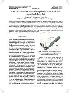
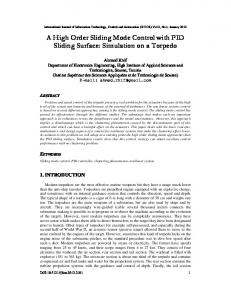
for all t E [ti, ti+d. Figs. 1 (a)-(d) show plots of states, sliding variable, con­ trol input and sampling interval of the system, respectively. It can be seen that states of the system converge and remain ultimately bounded and the same is true for sliding variable. However, for fixed quantizer the sliding mode occurs in the vicinity of sliding surface. The simulation is carried out for different quantization level and is shown that the ultimate bound decreases with decrease in sensitivity of the quantizer. Further, the Zeno execution of event triggering condition is avoided with selecting suitable parameters.

3.5

1.5

0.5 -1 -1.5 �--�---�--��-� o 10 15 20 25 30

-0.5 �--�---�--� o 10 15 20 25 30

(a)

(b)

Time (sec)

Time (sec)

10 ,---,----,---,---,,--,

0.5 ,-----,---�--�---, +

0.45

h'

j

-5

"2 � c3

-10

'oD ;:: ;.c:: p,

-15

2

:J)

-20

0.4

0.25 0.2 0.15

0.05

-30 �--�---�--��-� o 15 10 20 25 30

Timc (SCC) (c)

+ +

03

0.1 -25

+

+ 0.35

+

+ +

+ +

+ +

+

++

+ +

+

+

++

+ •

J\ * 10

15

Time

20

25

30

(d)

Fig. l. (a) Evolution of states of the system (b) sliding surface (c) event based control input and (d) sampling interval generated by executing event condition.

V.

CONCLUSION

In this paper, an event-triggering SMC with quantized measurement is proposed. We propose a event condition that guarantees stability of the system even with quantized states. We also discuss event design parameters such that no Zeno execution occurs and the inter execution times are lower bounded by some positive quantity. Numerical simulation is provided to verify the above analysis. REFERENCES [I] R. Brockett and D. Liberzon, "Quantized feedback stabilization of linear systems", IEEE Trans. Autom. Control, vol. 45, no. 7, pp. 1279-1289, 2000. [2] D. Liberzon and D. Nesic, "Input-to-state stabilization of linear systems with quantized state measurements", IEEE Trans. Autom. Control, vol. 52, no. 5, pp. 767-781, 2007. [3] D. Liberzon, "Hybrid feedbackstabilization of systems with quantized signals", Automatica, vol. 39, no. 9, pp. 1543-1554, 2003. [4] N. Elia and S. Mitter, "Stabilization of linear systems with limited information", IEEE Trans. Autom. Control, vol. 46, no. 9, pp. 13841400, 200l. [5] A. J. Astrom and B. Bernhardsson, "Comparison of riemann and lebesgue sampling for first order stochastic systems", Int. Con! De­ cision and Control, Dec. 2002.

[6] P. Tabuada, "Event-triggered real-time scheduling of stabilizing control tasks", IEEE Trans. Autom. Control, vol. 52, no. 9, pp. 1680-1685, 2007. [7] M. Mazo Jr. and P. Tabuada, "Decentralized event-triggered control over wireless sensor/actuator networks", IEEE Trans. Autom. Control, vol. 56, no. 10, pp. 2456-2461, 20II. [8] U. Premaratne, S. K. Halgamuge, and 1. M. Y. Mareels, "Event triggered adaptive differential modulation: a new method for traffic reduction in networked control systems", IEEE Trans. Autom. Control, vol. 58, no. 7, pp. 1696-1706, 2013. [9] A. K. Behera and B. Bandyopadhyay, "Event triggered robust sta­ bilization linear systems", in 40th IEEE Annual Con! of IEEE Ind. Electronics Soc., pp. 133-138, Oct-Nov. 2014. [10] A. K. Behera, B. Bandyopadhyay, N. Xavier and S. Kamal, "Event­ triggered sliding mode control for robust stabilization of linear mul­ tivariable systems", X. Yu and M. O. Efe (Eds.), Studies in Systems, Decision and Control, Springer, 2015. [ll] P. Tallapragada and N. Chopra, "On event triggered tracking for nonlinear systems", IEEE Trans. Autom. Control, vol. 58, no. 9, pp. 2343-2348, 2013. [12] J. Lunze and D. Lehmann, "A state-feedback approach to event-based control", Automatica, vol. 46, no. 1, pp. 2ll-215, 2010. [13] K. -E. Arien, "A simple event-based PID controller", in Preprints 14th World Congr. IFAC, Beijing, China, Jan. 1999. [14] V. T. Utkin, "Variable structure systems with sliding modes", IEEE Trans. Autom. Control, vol. 22, no. 2, pp. 212-222, 1977. [15] W. Gao, Y. Wang, and A. Homaifa, "Discret-time variable structure control systems", IEEE Trans. Ind. Electron., vol. 42, no. 2, pp. 117122, 1995.

[16] A. Bartoszewicz, "Discrete-time quasi-sliding-mode control strate­ gies", IEEE Trans. Ind. Electron., vol. 45, no. 4, pp. 633-637, 1998. [l7] S. lanardhanan and B. Bandyopadhyay, "Output feedback sliding­ mode control for uncertain systems using fast output sampling tech­ nique", IEEE Trans. Ind. Electron., vol. 53, no. 5, pp. 1677-1682, 2006. [18] B. Bandyopadhyay and S. lanardhanan, "Discrete-time sliding mode control- A multirate output feedback approach", Lecture Notes in Control and Information Sciences, Springer, 2005. [19] M. C. Saaj, B. Bandyopadhyay, and H. Unbehauen, "A new algorithm for discrete-time sliding-mode control using fast output sampling feed­ back", IEEE Trans. Ind. Electron., vol. 49, no. 3, pp. 518-523, 2002. [20] S. lanardhanan and B. Bandyopadhyay, "On discretization of continuous-time terminal sliding mode", IEEE Trans. Autom. Control, vol. 51, no. 9, pp. 1532-1536, 2006. [21] A. K. Behera and B. Bandyopadhyay, "Steady-state behavior of discretized terminal sliding mode", Automatica, vol. 54, pp. l76-181, Apr. 2015. [22] M. L. Corradini and G. Orlando, "Robust quantized feedback stabi­ lization of linear systems", Automatica, vol. 44, no. 9, pp. 2458-2462, 2008. [23] B.-C. Zheng and G.-H. Yang, "Robust quantized feedback stabilization of linear systems based on sliding mode control", Optim. Control Appl. Method, vol. 34, pp. 458-471, 2012. [24] B.-C. Zheng and G.-H. Yang, "Quantised feedback stabilisation of planar systems via switching-based sliding-mode control", lET Control Theory & Appl., vol. 6, no. 1, pp. 149-156, 2012. [25] S. Chakrabarty and B. Bandyopadhyay, "Quasi sliding mode control with quantization in state measurement", Ann. Con! Ind. Electrinics Soc., vol. 49, no. 3, pp. 3971-3976, 201l. [26] Y. Yan and X. Yu, "Quantization behaviors in equivalent-control based sliding-mode control systems", Advances in Sliding Mode Control, Lecture Notes on Control In! Science, B. Bandyopadhyay et. al (Eds.) pp. 221-224, 2013. [27] D. Lehmann and 1. Lunze, "Event-based control using quantized state information", 2nd IFAC Workshop on Distributed Estimation and Con­ trol in Networked Systems, DOI:IO.3182/20100913-2-FR-4014.00003, 2010.