works with: A set of fuzzy rules (not a fuzzy relation ... the FLC, the normalization limits and the MF. ... real numbers ranged in -1,1] (variables are normal- ized, then fuzzy sets must be de ned with the same range). Each row of the array contains ...
Evolutionary-Based Learning Applied to Fuzzy Controllers. Luis Magdalena, F�elix Monasterio ETSI Telecomunicaci�on, Universidad Polit�ecnica de Madrid, Ciudad Universitaria s/n., E-28040 Madrid, Spain. Abstract|Fuzzy Logic Controllers constitute knowledge-based systems that include fuzzy rules and fuzzy membership functions to incorporate the human knowledge into their knowledge base. The de nition of fuzzy rules and fuzzy membership functions is actually a�ected by subjective decisions, having a great in uence over the whole FLC performance. Some e�orts have been made to obtain an improvement on system performance by incorporating learning mechanisms to modify rules and/or membership functions. Genetic Algorithms (GAs) are probabilistic search and optimization procedures based on natural genetics. This paper proposes a new way to apply GAs to FLCs, and applies it to a FLC designed to control the Synthesis of biped walk of a simulated 2-D biped robot.
I. INTRODUCTION
Fuzzy Logic Controllers [1] (FLCs) are being widely and successfully applied to di�erent areas. FLCs are knowledge-based systems that include fuzzy rules and fuzzy Membership Functions (MF) to incorporate the human knowledge into their knowledge base. The de nition of fuzzy rules and fuzzy MF is actually a�ected by subjective decisions, having a great in uence over the whole FLC performance. Some e�orts have been made to improve system performance by incorporating learning mechanisms to modify rules and/or MF. The application of Genetic Algorithms (GAs) to FLCs in such a way has recently produced some interesting works [2]-[7]. GAs are probabilistic search and optimizationprocedures based on natural genetics, working with nite strings of bits that represent the set of parameters of the problem, and with a tness function to evaluate each one of these strings. This paper proposes a new way to apply GAs to FLCs with some special characteristics like a large number of variables or unknown (or changing) ranges for the variables of the controller.
II. GA'S AND FLC'S.
A. Genetic Algorithms.
GAs are search and optimization techniques that are based on natural genetics, and are usually characterized by:
1. A coding scheme for each possible solutions of the problem, using nite strings of bits (each string will be called chromosome and each bit will be referred to as a gene). 2. An evaluation function that estimates the quality of each solution (each string) that compose the set of solutions (called population). 3. An initial set of solutions to the problem (initial population). 4. A set of genetic operators that using the information contained in a certain population (referred to as a generation) and a set of genetic parameters, creates a new population (the next generation). 5. A termination condition to de ne the end of the genetic process. The Genetic process has the following structure: 1. Start with a population that constitutes the rst generation G(0). 2. Evaluate G(0): taking each string (chromosome) of the population, decoding it, evaluating it by means of the evaluation function, and assigning a tness value to the string. 3. While the termination condition was not met, do (a) Create a new generation G(t+1), by applying the genetic operators to the generation G(t). (b) Evaluate G(t+1). 4. Stop. The basic genetic operators (used by the GAs enumerated along the next Subsection) are three: reproduction, crossover and mutation. The reproduction operator creates a mating pool where strings copied (or reproduced) from G(t) await the action of crossover and mutation. Those strings from G(t) with a higher tness value, obtains a larger number of copies in the mating pool. The crossover operator provides a mechanism for strings to mix attributes through a random process. This operator is applied
to pairs of strings from the mating pool, and has three steps: a pair of strings is randomly selected from the mating pool, a position along the string is selected uniformly at random, the bits following the crossing site are swapped between both strings. Mutation is the occasional alteration of a gene at a certain string position. Each gene is a candidate for mutation and will be selected according to a mutation probability. B. GAs applied to FLCs.
GAs enumerated in this Subsection follows the general ideas previously described, using its own coding scheme. Some of these works use strings of numbers instead of strings of bits. The evaluation function, the rst generation (initial population) and the termination condition are related with the task to which each FLC was designed for. When modifying MF, usually triangular or trapezoidal functions are employed. These functions are parameterized with one to four coe�cients and each of these coe�cients will constitute a gene of the chromosome for the GA. This gene may be a binary code (representing the coe�cient) [2, 3, 4] or a real number (the coe�cient) [5]. In [6], GAs are used to modify the decision table of a FLC, which is applied to control a system with two input and one output variables. A chromosome is formed from the decision table by going rowwise and coding each output fuzzy set as an integer in 0, 1, : : :, n, where n is the number of MF de ned for the output variable of the FLC. Value "0" indicates that there is no output, and value "k" indicates that the fuzzy set has the k-th membership function. The system includes an elite strategy under which the best solution at a given generation is promoted directly to the next. Occasionally GAs are used to modify the fuzzy relational matrix (R) of a one input, one output FLC. The chromosome is obtained by concatenating the m � n elements of R, where m and n are the number of fuzzy sets associated with the input and output variable respectively. The elements of R that will make up the genes may be represented by binary codes [7] or real numbers [5]. All these works propose really interesting ways to add learning capabilities to a FLC by means of a GA, obtaining results that show the ability of GAs to improve the performance of prede ned FLCs. We nd out on the application examples of these works, FLCs with two to ve variables (input and output) and up to twenty MF (adding those from each variable). The question is how do they work when the problem dimensions will increase. A new approach that uses a di�erent coding strategy to avoid the problems that will probably produce larger dimension FLCs is proposed in the next Section.
III. CODING THE INFORMATION
As pointed out by di�erent authors, when applying GAs to FLCs, there are two basic decisions to be made: how to code the possible solutions to the problem as nite bit string, and how to evaluate the merit of each string. This Section will present the coding scheme that uses the learning system, starting by describing some design characteristic of the FLC, that de nes the kind of information to be encoded. The learning system will be applied to a FLC that works with: A set of fuzzy rules (not a fuzzy relation matrix or a fuzzy decision table) Input and output variables linearly normalized on [-1,1] (from its real range [vmin; vmax ]). Fuzzy sets with trapezoidal MF de ned through four parameters. The Knowledge Base of the FLC contains the information to be coded, and is divided into a Data Base and a Rule Base. From the view point of encoding, the Data Base contains three di�erent informations: a set of parameters, a set of normalization limits and a set of MF, and the Rule Base contains a set of fuzzy control rules. Classical GAs operate on xed-length binary strings. Our system will break that restriction, working on the unconstrained area of Evolution Programs (EP) [8]. The idea of evolution programs is entirely based on GAs, but allowing any data structure with any set of "genetic" operators. The counterpart of the use of an unconstrained encoding scheme, is the need of de ning new code-adapted "genetic" operators. A. Encoding the Data Base information.
Three elements must be encoded: the parameters of the FLC, the normalization limits and the MF. The set of parameters de nes the dimensions of the system, that is, the number of input variables (N) and output variables (M), and (assembled on the vectors n and m) the number of linguistic terms (or the number of fuzzy sets) associated with each member of the set of input variables and output variables. The i-th component of vector n (n = fn1; : : :; nN g) represent the number of linguistic terms associated with the i-th input variable. The j-th component of vector m (m = fm1 ; : : :; mM g) is the number of linguistic terms associated with the j-th output variable. An array of (N + M) � 2 real numbers will represent the set of normalization limits. Each row of this array contains the limits of a system input or output variable (fvmin; vmax g). The set of MF, contains the MF of L fuzzy sets, where L could be obtained from n and m as shown in the following equation: La =
XN ni ; Lc = XM mj ; L = La + Lc: i=1
j =1
(1)
This set will be represented by an array of L � 4 real numbers ranged in [-1,1] (variables are normalized, then fuzzy sets must be de ned with the same range). Each row of the array contains the four parameters that describe a trapezoidal fuzzy set. We can obtain a string of reals by concatenating the rows of this array as it has been made in some works presented in previous Section.
and the union of the fuzzy sets de ned for the input variable, generates a fuzzy set whose membership function is equal to one for any input value. The number of elemental rules replaced by a certain rule is obtained by multiplying the number of rules replaced for each variable. Considering a FLC with parameters N = 3; M = 1; n = f5; 3; 5g and m = f7g (La = 13; Lc = 7), the fuzzy rule
B. Fuzzy rules representation.
x1 is (C13 or C14) and x3 is (C31 or C32) y1 is (D14 or D15) (4) replaces 2 � 3 � 2 = 12 elemental fuzzy rules. When the FLC works with a few input variables (like those described on Section II), the fuzzy relation matrix or the fuzzy decision table allow an adequate encoding of the knowledge to be used by the GA. When the number of input variables increases, the decision table grows exponentially. The number of elemental rules grows at the same rate. The rules obtained when acquiring the knowledge from the experts, usually contains subsets of the input variables (no more than four or ve input variables each rule) as shown in [9, 10] and then, the number of elemental rules replaced by each rule increases exponentially too. As a consequence the dimension of the set of rules shows a considerably slower growing rate than the dimension of the elemental fuzzy rules set. As a counterpart of this important advantage, the set of rules may arise in problems like incompleteness or inconsistency. These problems may be treated through an adequate design of the FLC to avoid them, or including some consistency and completeness criteria in the learning strategy (usually into the evaluation function). Our conclusion is that a fuzzy rule representation will probably remain treatable for the GA, when the decision table representation has became untreatable.
When applying GAs to FLCs, rules are generally represented as fuzzy decision tables or fuzzy relational matrix. Our system will work directly with the set of fuzzy rules. The fuzzy system may be characterized by a set of fuzzy rules combined with the sentence connective also [1]: R = also (R1; R2; : : :; Rk): When working with a multiple input system, decision tables become multidimensional. A system with three input variables produces three-dimensional decision tables. The number of "cells" of these decision tables is obtained by multiplying the number of linguistic terms associated with each input variable. Using the previous de nitions of n and N, the number of "cells" (Lr ) is: Lr =
YN ni
i=1
(2)
Each cell of the table describes a fuzzy rule, we will refer to these fuzzy rules as elemental fuzzy rules. The structure of the fuzzy control rules contained in our FLC with parameters fN; M; n; mg is: If xi is Cio and : : :and xk is Ckp (3) then yj is Djq and : : :and yl is Dlr where xi is an input variable, Cio is a fuzzy set associated with this variable (o � ni ), yj is an output variable and Djq is a fuzzy set associated with this variable (q � mj ). All fuzzy inputs are 'connected' by the fuzzy connective 'and'. Several fuzzy sets related with the same variable and connected with the aggregation operator 'or', may appear in a single rule like: If xi is(Cio or Cip) and : : : then yj is(Djq or Djr ) : : : These rules are not elemental fuzzy rules, an elemental fuzzy rule must contain fuzzy inputs for all of the input variables, and not 'or' operators. A rule containing an 'or' operator, replaces two elemental fuzzy rules (the rule is equivalent to the aggregation of the elemental rules when working with the connective also as the union operator). A rule that has no fuzzy input for a certain input variable, replaces as many elemental rules as the number of fuzzy sets de ned for the input variable. The rule is equal to the aggregation of the elemental rules when: working with the connective also as the union operator,
If then
C. Encoding the Rule Base information.
A set of rules represented by numerical values on a decision table or a relation matrix, have a direct translation into a string by a concatenating process. This method does not apply to a set of rules with a structure like that de ned by equation 3. In our system, each rule will be encoded into two strings of bits: one string of length La for the antecedent (a bit for each linguistic term related with each input variable) and one string of length Lc for the consequent. To encode the antecedent we will start with a string of La bits all of them with an initial value 0. If the antecedent of the rule contains a fuzzy input like xi is Cij , a 1 will substitute the 0 at a certain position (p) of the string: p=j+
Xi?1 nk:
k=1
(5)
This process will be repeated for all the fuzzy inputs of the rule. It is important to point out that using this code, an input variable for which all the corresponding bits have value 0, is an input variable whose value has no e�ect over the rule. The process to encode the consequent is quite similar to that described above. Starting with a string of Lc bits all of them with an initial value 0, a fuzzy output like yi is Dij , will be encoded by passing to 1 the bit at position q of the string (the second string):
Xi?1 q = j + mk :
The e�ect produced by the modi cation of the normalization limits of a certain variable on the corresponding fuzzy sets (MF) are two: shrinkage or expansions and shifting to the right or left. This changes are restricted from those obtained with other methods, but the length of the employed code is reduced substantially, producing a shorter learning process; and a shorter or larger process may produce a treatable or untreatable problem. B. The evolution operators.
(6) A part of evolution operators is obtained by directly adapting the classical genetic operators to the code. k=1 Others are new operators taking advantage of the In this case, when all the bits corresponding to an code structure, or reducing its disadvantages. output variable have value 0, the rule has no e�ect 1) Reproduction: The reproduction operator over that output variable. starts with an elite process that may be de ned on The rule described in 4 is encoded as the basis of a number of members, a percentage of 0011000011000 - 0001100: (7) members or an evaluation threshold ( xes or variables). By this process, a subset of G(t), referred Each rule of this FLC will be represented as a string as the elite of generation t (E(t)), will be directly of 20 bits ( xed length). The rule base will contain reproduced (copied) on G(t + 1). an un xed number of rules, with a maximum value In a second step, individuals of G(t) will be copied of Lr = 75, then it will be encoded as a string of up to the mating pool with a possibility criterion based to 75 strings of 20 bits. on the tness of each one. According to the classical reproduction operator, members with larger tness IV. EVOLUTION LEARNING value receive a larger number of copies. This operaThe process of evolution learning may be described tor has been slightly modi ed: members (including with the same scheme that the genetic process of those from the elite) with larger tness value have Subsection II.A. The keys of this process are: the a higher possibility to receive a single copy (each code, the evaluation function, the termination condi- individual receives or not a copy). tion and the evolution operators. The code has been Once the elite and the chromosomes to be reprowidely presented along the previous section and will duced have been selected, the number of members be summarized here. The evaluation function and of G(t + 1) must be adjusted to the maximum popthe termination condition are application speci c. ulation. This process is performed by adding new The main question for this section are the evolution elements to the elite (if the number of memebers operators, or in a more general sense, the creation is under the maximum population) or by extracting chromosomes from the mating pool (if the number of G(t + 1) from G(t). of members is over the maximum population). A. The code. 2) Crossover: Once a pair of parents (mi and The code that contains the information of the knowl- mj taken from the mating pool) has been selected to edge base is: be crossed ( rst step of the process), the crossover 1. A string of 2 + N + M integers containing the operator produces two new chromosomes by mixing the information provided by parents genes. A set of dimensions of the FLC. strings contains this information, two strings in our 2. A string of (N +M) � 2 real numbers containing case (Normalization limits and Rules). The inforthe normalization limits of the variables. mation contained on each string is not independent, then, if possible, the operator must work simultane3. A string of (La +Lc ) � 4 real numbers containing ously (and not independently) on both strings. Each the de nition of the trapezoidal MF. chromosome is composed by a pair of subchromo4. A string of up to Lr rules, where each rule is a somes encoding the rule base (r) and the data base (d). The crossover of mi = (ri ; di) and mj = (rj ; dj ) string of La + Lc bits. will produce two new chromosomes (mu and mv ). It is possible to apply the evolution learning to Rule base subchromosomes have not xed length, any part of this code, according with the conditions and their genes are rules: of the learning process. From this point and on the application example we will work only with normalri = fri1; : : :; rik g (8) ization limits (2) and with rule bases (4). rj = frj 1; : : :; rjlg:
To cross ri and rj a cutting point must be selected for each string. Since the lengths of the strings may not be equals, cutting points ( and ) will be obtained independently for ri and rj ri = fri1; : : :; ri jri +1; : : :; rikg (9) rj = frj 1; : : :; rj jrj +1; : : :; rjlg; producing the new rules ru = fri1; : : :; ri jrj +1; : : :; rjlg (10) rv = frj 1; : : :; rj jri +1; : : :; rikg: After rule bases are crossed, the process of crossing data bases will consider what rules from ri and rj goes to ru or rv . An elemental fuzzy rule contains fuzzy inputs for all the variables. The rules we use contain fuzzy inputs and fuzzy outputs for only a subset of the input and output variables, then, normalization limits for the remaining variables have no in uence on the meaning of the rule. A larger in uence of a certain variable on rules that proceeding from ri go to ru, will produce a higher possibility for this variable to reproduce in du its corresponding range from di. The in uence is evaluated by simply counting the number of rules that containing the variable, are reproduced from ri to ru . The process of selection is independent for each variable and for each descendent (mu and mv ), consequently it is possible for both descendent to reproduce a certain range from the same antecedent. 3) Rules reordering: When a fuzzy system is characterized by a set of fuzzy rules, their ordering is immaterial, the sentence connective also has properties of commutativity and associativity. When concatenating decision tables or relation matrices, the information of a certain gene depends on its content and its position. In our string of rules, the meaning of a gene becomes independent of the position. Therefore, since rule position is arbitrarily de ned for the members of the rst population, and it is immaterial for the output, an operator to reorder rules will be added to the system. This operator applies to each set of rules produced by crossover operator, with a probability de ned as a parameter of the evolution system. To reorder a rule base (ri ) a cutting point ( ) is selected uniformly at random, to create a new rule base (rj ) ri = fri1; : : :; ri jri +1 ; : : :; rikg (11) rj = fri +1 ; : : :; rikjri1; : : :; ri g: The operator has no e�ect over the data base. 4) Mutation: The mutation is composed of two di�erent processes: rule mutation and range mutation. The rule mutation process will work at the level of bits that compose a rule. Each rule is composed of (La + Lc ) bits and has the structure p11 : : :p1n1 : : :pN 1 : : :pNnN (12) c11 : : :c1m1 : : :cM 1 : : :cMmM
where pij is the bit related to j-th fuzzy set of the i-th input variable, and cij is the bit related to j-th fuzzy set of the i-th output variable. The rule mutation operator works as the classical genetic mutation applied to the string of bits de ned by equation 12. This operator di�ers from classical mutation because it does not work at the level of genes (rules), but with the simplest element (bits) that compose genes. The range mutation process has two di�erent definitions: one for those variables that have a symmetrical range whose mutation will produce a symmetrical range, and other for the rest. If a certain variable has the range [�l ; �u], the mutation process could be described by the following equation If �l (t) = ?�u (t) �l (t + 1) = (1 + KPS)�l (t) �u(t + 1) = (1 + KPS)�u (t) If �l (t) 6= ?�u (t) �l (t + 1) = �l (t) + KP1S1 (�u (t) ? �l (t)) �u(t + 1) = �u (t) + KP2S2 (�u (t) ? �l (t)); (13) where K 2 [0; 1] is a parameter of the learning system that de nes the maximum variation (shift, expansion or shrinkage). P, P1 and P2 are random values uniformly distributed on [0; 1], and S, S1 and S2 take values -1 or 1 by a 50% chance.
V. AN APPLICATION EXAMPLE
This section shows an example of application of the learning strategy to a FLC. The FLC task will be the Synthesis of Biped Walk, of a simulated 2-D biped robot. The most interesting characteristics of biped systems are: An unpowered degree of freedom (d.o.f.) formed between the contact of the foot and the ground surface. A certain repeatability of movements. Permanent changes between double, single and none-support phases (2, 1, 0 feet in contact with the ground). The presence of a closed kinematic chain in the double-support phase. A. The simulated biped robot.
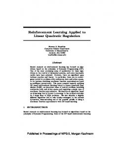
The simulated biped robot is a six-links 2-D structure with two legs a hip and a trunk. Each leg has a punctual foot, a knee with a degree of freedom and a hip with another degree of freedom. The model dimensions are shown in TABLE I. Fig. 1 shows variables used by the FLC (�1-�6), and the Mathematical Model (�1 -�6 ). Relations between both sets of variables are: ~� = [R]~� + ~r: (14) The dynamic equation for the model is represented by the following set of nonlinear di�erential equations �� = D(�)~� + C(�;_ �)~�_ + �(�); (15)
Table I MODEL DIMENSIONS
Link Length (m) Weight (kg) Trunk 0.65 35 Hip 0.10 7 Thigh 0.50 9 Shank 0.50 5
1
C1
-1
C2
C3
C4
C5
C6
C7
C8
C9
Fig. 2. Fuzzy sets.
variables are linearly normalized in [-1,1]. From the view point of learning process, those variables that where � are generalized forces. Considering ( 14) we are simultaneously input and output variables, have obtain a single range. Consequently, crossover and muta�� = [R]T �� (16) tion of ranges work over a set of 22 ranges. and characterize the presence of the unpowered d.o.f. C. The initial knowledge. by (17) The data base contains the description of normalized ��1 = 0: fuzzy sets (on this application example we will use a From 15, 16 and 17, the second-order di�erential single description, Fig. 2, for all the variables) and equation the normalization limits for each variable. The Initial knowledge for the fuzzy system has A1 �1 +A2 (�_1 )2 +A3 �_1 +A4 cos �1 +A5 sin �1 +A6 = 0 been derived from biomechanical studies [11, 12]. (18) Working with this knowledge we obtain the normalis obtained and then solved by Runge-Kuta method. ization limits for each input and output variable and Coe�cients A1 to A6 are function of �2 ; �_2; �2 to the initial set of fuzzy rules. A sample of fuzzy rule �6 ; �_6 ; �6. is: If Support is Single B. Characteristics of the FLC. and Center of gravity position (CGx ) is negative or zero (C1 orC2 orC3 orC4 orC5 ) The characteristics of the FLC are: and Stance-leg hip position (�3 ) is Negative small (C4 ) Compositional operator: sup-min. and Stance-leg hip velocity (�_3 ) is Negative Fuzzy implication function: Larsen's product. ( C orC 1 2 orC3 orC4 ) The union operator as connective 'also'. then Stance-leg hip velocity (�_3) is zero (C5 ) Defuzzi cation strategy: center of area. and Stance-leg hip acceleration (�3) is zero (C5 ) The parameters of the FLC are: Input variables (N): 22. VI. RESULTS Output variables (M): 15. Fuzzy sets per variable (ni , mj ): 9. The evolution learning process will be applied to the Control cycle of 0.01 sc. FLC that controls the gait synthesis. A chromosome Its 22 input variables are position, velocity and will contain a set of fuzzy rules and a set of normalacceleration for each d.o.f including the unpowered ization ranges. This information will be referred to one (�1 to �6 of Fig. 1) and for the horizontal as a gait description or a gait pattern. When the component of the center of gravity (CGx) of the me- information encoded by a chromosome is used by chanical structure, and a binary variable represent- the FLC, a sequence of movements is produced on ing the single or double support phase. Its 15 output the biped. This sequence of movements will be evalvariables are position, velocity and acceleration for uated, based on the stability and regularity of the each powered d.o.f. (�2 to �6). Input and output walk, over a 10 seconds simulation (a thousand control cycles, from ve to twenty steps). Some chromosomes will contain valid gait patterns, that is, gait description that produces a walk simulation without falling or stopping the biped, these gait patterns may δ α be characterized by its walking parameters: speed, δ α δ α stride length and frequency. The evolution process starts with an initial popuδ α δ lation of chromosomes and has the objective of proα ducing a set of valid gait patterns with di�erent parameters, not the best gait pattern. This set of gait δ α patterns will allow the biped to walk with di�erFig. 1. System and model variables. ent speed or frequency. Following the objective, the
1
elite will contain not the chromosome encoding the best gait pattern, but those that encode valid gait patterns. With the same idea, the termination condition will be de ned not in terms of evaluation of the best, but in terms of number or rate of di�erent valid patterns. Starting with a small population composed of a few valid patterns and a set of bad patterns the learning system has been tested with di�erent learning parameters. Each simulation has produced new gait patterns with di�erent gait parameters: frequency, speed and length (only two of them are independent). Results of learning processes without mutation, displayed on the space of gait parameters, are shown in Fig. 3 and 4. The gures show the relation between stride length (m) and walking speed (m=sc) for a set of gait patterns. Each square place (on the space of gait parameters) a valid pattern of the population, solid ones are those remaining from the rst population. These results correspond to generation 25 and are obtained starting with a rst population of 27 individuals (5 valid and 22 bad patterns), using a crossing rate of 0.8, and working with a maximum population of 500 (Fig. 3) and 100 (Fig. 4) individuals respectively. The results of adding the mutation operator to the previous processes are shown in Fig. 5 (after 41 generations) and 6 (after 32 generations). The ranges mutation rate is set to 0.05. The value of K on equation ( 13) is set to 0.5. The initial population, and other learning parameters remain unchanged.
VII. CONCLUSIONS
The main goal of this work was the de nition of a learning methodology based on evolution, to be applied to FLCs. Some previous works that introduced GAs based learning on FLCs have been summarized (GA is a type of evolution system). A new approach adapted to systems with a larger number of variables have been proposed and tested over a FLC controlling a complex problem, the locomotion of a simulated six-links biped robot. The objective of the learning system was obtaining new gait patterns (with di�erent gait parameters) by applying the learning techniques to a set of prede ned ones. Figures 3 and 4 show some simulations that start with a set of patterns whose speed was ranged in the interval [1:05; 1:15]m=sc, and have produced a new set of patterns with a wider range of speeds ([0:88; 1:23]m=sc). Adding a mutation operator, the e�ect of the evolution learning is magni ed as show in gures 5 and 6 where the range of speeds is [0:55; 1:23]. The objective was obtaining new gait patterns, but during this process, the system has produced gait descriptions with higher evaluation value than the previous existing. The higher evaluation from a member of the rst generation was 0.9491 (maximum evaluation 1) and 0.8
the next one, nal population of the experiment presented on Figure 5 has produced a best evaluation of 0.9817, and 49 other gait patterns evaluated over 0.9491 (the best proceeding from initial knowledge). These fty evolution-generated gait patterns are distributed on the space of parameters as show on Figure 7. Obviously this is only the rst step of the analysis, and a deeper study that includes the dependence of learning on initial knowledge, maximum population and other learning parameters is needed. However, presented results show that the proposed method is a valid way to add learning capabilities on FLC with a large number of variables.
References
[1] Lee C.C., "Fuzzy Logic in Control Systems: Fuzzy Logic Controller, Part I-II, IEEE Transactions on Systems, Man and Cybernetics, vol 20, num 2, pp 404-435. Mar/Apr. 1990. [2] Karr C.L., "Design of an Adaptive Fuzzy Logic Controller Using a Genetic Algorithm", Proceedings 4th. International Conference on Genetic Algorithms, pp 450457. Morgan Kaufmann, 1991. [3] Karr C.L. and Gentry E.J., "Fuzzy Control of pH Using Genetic Algorithms". IEEE Transactions on Fuzzy Systems, vol 1, num 1, pp 46-53. Feb. 1993. [4] Lee M.A. and Takagi H., "Integrating Design Stages of Fuzzy Systems using Genetic Algorithms", Proceedings Second IEEE International Conference on Fuzzy Systems, FUZZ-IEEE'93, vol 1, pp 612-617. Mar. 1993. [5] Park D., Kandel A. and Langholz G., "Genetic-Based New Fuzzy Reasoning Models with Application to Fuzzy Control", IEEE Transactions on Systems, Man and Cybernetics, vol 24, num 1, pp 39-47. Jan. 1994. [6] Thrift P., "Fuzzy Logic Synthesis with Genetic Algorithms", Proceedings 4th. International Conference on Genetic Algorithms, pp 509-513. Morgan Kaufmann, 1991. [7] Pham D.T. and Karaboga D., "Optimun Design of Fuzzy Logic Controllers Using Genetic Algorithms", Journal of Systems Engineering, pp 114-118. SpringerVerlag, 1991. [8] Michalewicz Z., Genetic Algorithms + Data Structures = Evolution Programs. Springer-Verlag, 1992. [9] Magdalena L., Velasco J.R., Fernandez G. and Monasterio F., "A Control Architecture for Optimal Operation with Inductive Learning", Preprints IFAC Symposium on Intelligent Components and Instrument for Control Applications, SICICA'92, pp 307-312. May .1992. [10] Magdalena L. and Monasterio F., "Fuzzy controlled gait synthesis for a biped walking machine", Fuzzy Logic Technology & Applications, pp 117-122, ed. R.J. Marks II. IEEE Press 1994. [11] McMahon T., "Mechanics of locomotion". International Journal of Robotics Research, vol 3, num 2, pp 4-28. 1984. [12] Plas F., Viel E. et Blanc Y., La marche humaine, MASSON, S.A. Paris, 1984.
Fig. 3. Generation 25. Large population.
Fig. 4. Generation 25. Small population.
Fig. 5. Mutation with large population.
Fig. 6. Mutation with small population.
Fig. 7. Best evolution generated gait patterns.