Evolutionary Programming for the Length Minimization of ... - Lania

Evolutionary Programming for the Length Minimization of Addition Chains Sa´ ul Dom´ınguez-Isidroa , Efr´en Mezura-Montesa,∗, Luis Guillermo Osorio-Hern´andezb a

Department of Artificial Intelligence School of Physics and Artificial Intelligence University of Veracruz Sebasti´ an Camacho 5, Centro, Xalapa, Veracruz, 91000, MEXICO. b National Laboratory of Advanced Informatics (LANIA) A.C. R´ebsamen 80, Centro, Xalapa, Veracruz, 91000, MEXICO.

Abstract This paper presents the use of evolutionary programming to minimize the length of addition chains. Generating minimal addition chains is considered an NP-hard search problem. Addition chains are employed to reduce the number of multiplications in modular exponentiation for data encryption and decryption in public-key cryptosystems. The algorithm is based on a mutation operator able to generate a set of feasible addition chains from a single solution and a replacement mechanism with stochastic elements to favor diversity in the population. Furthermore, the proposed algorithm is coupled with a deterministic method with the aim to solve large exponents. Five experiments are carried out to test the approach in different types of exponents. The proposed algorithm is able to find competitive or even better results by requiring a lower number of evaluations with respect to those required by state-of-the-art nature-inspired algorithms. Keywords: Evolutionary Algorithms, Evolutionary Programming, Optimization, Addition Chains

∗

Corresponding Author. Phone: +52 228 8172957 Fax: +52 228 8172855 Email addresses: [email protected] (Sa´ ul Dom´ınguez-Isidro), [email protected] (Efr´en Mezura-Montes), [email protected] (Luis Guillermo Osorio-Hern´ andez)

Preprint submitted to Engineering Applications of Artificial IntelligenceSeptember 11, 2014

1. Introduction In most public-key cryptosystems such as Rivest-Shamir-Adleman (RSA) (Rivest et al., 1978), Diffie-Hellman (Ryabko and Fionov, 2005), ElGamal (ElGamal, 1985), Digital Signature Algorithm (DSA) (Ryabko and Fionov, 2005) and others, modular exponentiation or field exponentiation is used in the process of data encryption and decryption. Modular exponentiation consists of calculating a natural exponentiation and then computing the modulus on a number p (Bola˜ nos and Bernal, 2008) as follows: b ≡ ae mod p

(1)

where a is a positive integer in range [0, 1, 2, ..., p-1], e is an arbitrary positive number, and p is a prime number. The main benefit of modular exponentiation in cryptography is the use of very large exponents up to 1024 bits. However, the exponentiation operation (ae ) in Equation 1 is computationally expensive for larger exponents. There are two main ways to deal with such problem: (1) to increase the speed of the operation by means of distributed or parallel computing with highspeed processors, or (2) to reduce the number of multiplications required to compute the exponentiation operation. This work focuses on the second way to decrease the computational cost of exponentiation, specifically by using addition chains (Wu et al., 2006). An addition chain U with length L(U ) is defined as a sequence of positive integers U = u1 , u2 , . . . , ui , . . . , ul where u1 = 1, u2 = 2, ul = e, and ui−1 < ui < ui+1 < . . . < ul , where each ui is obtained by sum of two previous elements in the chain (not necessarily different) ui = uj + uk where j, k < i for i > 2. In other words, an addition chain U with length L(U ) is a sequence of numbers that satisfies the following properties: • The first number is 1. • Each number is generated by the addition of two previous numbers. • The exponent e appears at the end of the chain. An addition chain (AC for short) is then an option, based on the rules of exponents, to reduce the number of multiplications in an exponentiation operation. As an example, to compute a77 , 77 multiplications are originally 2

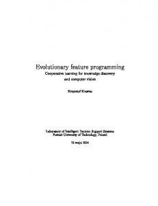
Figure 1: Differences between an addition chain and an Euclidean addition chain

required. Instead, with the following AC: [1 → 2 → 4 → 5 → 9 → 18 → 36 → 72 → 77] it can be accomplished with only 8 multiplications, as follows: a → a2 = a.a → a4 = a2 .a2 → a5 = a4 .a1 → a9 = a5 .a4 → a18 = a9 .a9 → a36 = a18 .a18 → a72 = a36 .a36 → a77 = a72 .a5 The length of an AC is then the number of multiplications required for an exponentiation operation. However, for a single exponent e different ACs can be generated. Furthermore, finding an AC with minimal length is considered an NP-Hard problem (Bos and Coster, 1990; Kaya-Koc, 1994). A particular type of addition chain is the Euclidean addition chain (EAC), where doubling of numbers is not allowed, i.e., a number within the EAC comes from the sum of two previous and different numbers. See Figure 1 for a graphical example of the difference between an AC and an EAC. EACs are useful in data encryption and decryption processes in publickey cryptosystems because they help to prevent diverse types of attacks, such as side channel attacks (e.g., simple power analysis and differential power analysis), safe error attacks and fault attacks (Fumaroli and Vigilant, 2006; Joye, 2009; Lawson, 2009; Quisquater and Koene, 2002; Herbaut et al., 2010). The methods to find minimal length ACs can be roughly divided into: (1) deterministic and (2) stochastic approaches (Cruz-Cort´es et al., 2008). Among the most popular deterministic methods there are the following: The binary method consists of strategies which expand the exponent e to its binary representation. The binary chain is scanned bit by bit from left to right. For each bit scanned, the current value of the AC is multiplied by 2. 3

If the current bit is one, it is then added to the current value of the AC. This process is repeated until all the binary string is covered. The binary method works with the Hamming weight of e (Kaya-Koc, 1994; Van-Der Kruijssen, 2007). The factor method is based on the factoring in the multiplication rules and it is divided in two stages: In the first stage, a tree of integers is constructed, in which for each parent node n, the child nodes are the factoring of n. The construction of the tree ends when child nodes have a value of 1. The second stage of the method consists of traversing the tree to build the AC. Further explanations can be found in (Knuth, 1981; Van-Der Kruijssen, 2007). The window method is based on k-ary expansion of the exponent e, where exponent bits are divided into k -bit words or windows (Kunihiro and Yamamoto, 1998). Each window has a maximum length which has to be defined by the user. The resulting words are scanned by performing consecutive squarings and a subsequent multiplication as needed. For k = 1, 2, 3 and 4 the window method is called, binary, quaternary, octary and hexa exponentiation method, respectively. A more detailed explanation can be found in (Kaya-Koc, 1994). The sliding window method (SWM) significantly outperforms the window method mentioned before and it is useful for very large exponents. SWM splits the exponent e in zero and non-zero windows. This window separation streamlines the ACs generation as indicated by Kaya-Koc (1994). On the other hand, there are recent research works on stochastic methods to find minimal length ACs. Three different nature-inspired techniques are distinguished: (1) swarm intelligence, (2) artificial immune system (AIS) and (3) genetic algorithm (GA). They are described below. In (Nedjah and de Macedo-Mourelle, 2006), the authors adapted the Ant Colony Optimization (ACO) (Dorigo et al., 1996) to generate short ACs. ACO is based on a multi-agent schema, where each agent represents an ant. To improve ACO’s capabilities on this particular problem, two types of memories were added to the approach: shared memory and local memory. Only a few exponents were tested in this approach. Particle Swarm Optimization (PSO) was also used to find minimal length ACs for different types of exponents (Le´on-Javier et al., 2009). Each particle represented an AC and the velocity vector was transformed into a velocity chain, where the value at each position in that vector represented the preceding value used to generate each number in the particle, i.e., the AC. The Artificial Immune System (AIS) was modified in (Cruz-Cort´es et al., 4

2008) to deal with ACs. AIS algorithm emulates the pattern matching abilities between antibodies and antigens and the emergence of a behavior to detect foreign cells in the body (Nunes de Castro and Timmis, 2002). Based on the clonal selection principle those better solutions, i.e., those shorter ACs, are cloned and then mutated. The use of GAs has been also reported in the length minimization of addition chains. In (Cruz-Cort´es et al., 2005) one-point crossover and uniform mutation were employed, while in (Osorio-Hern´andez et al., 2009) two-point crossover, a local-search mutation operator and a repair mechanism used in the initialization of the population were joined in a GA. The second version (Osorio-Hern´andez et al., 2009) outperformed the results of the first one (Cruz-Cort´es et al., 2005). Moreover, Rodriguez-Cristerna and TorresJimenez (2013) proposed a GA which includes a representation based on the factorial number system, a blend of neighborhood functions and a blend of distribution functions. The approach was not tested with large exponents. The literature review above shows that, besides deterministic methods, nature-inspired algorithms have been adapted to find minimal length ACs. However, there are other evolutionary algorithms which remain unexplored. This is the main motivation of this work, where evolutionary programming (EP) is adapted to find ACs with minimal length. EP is attractive for different reasons: (1) It is a very simple evolutionary algorithm because it only uses mutation as a variation operator to generate new individuals (solutions of the problem being solved). Moreover, it usually does not require a parent selection mechanism, i.e., all individuals generate offspring. Finally, its replacement mechanism is very simple to implement. A suitable solution encoding and fitness function, an adequate initial population generation mechanism, a special mutation operator, and a replacement mechanism to favor diversity in the population are added to EP to tackle the minimal length AC problem. The proposed algorithm is tested on sets of exponents with different features (including EACs) and it is also hybridized with the sliding window method to solve the problem with larger exponents. The contents of this paper are organized as follows: in Section 2 the EP algorithm is introduced while in Section 3 the adapted EP to deal with ACs is presented. Section 4 includes the experimental design, the results obtained and the corresponding discussion. After that, Section 5 covers the combination of the proposed algorithm with a deterministic method to deal with large exponents and the corresponding experiment is carried out. Finally, in 5

Section 6 some conclusions are drawn and the future work is established. 2. Evolutionary programming EP was proposed by Fogel in 1960 to optimize finite state machines, where the inheritance relationship and behavior between parents and offspring was highlighted (Fogel, 1999). Adaptation in this EA is conceived as a kind of intelligence. EP simulates the evolution at species level. Therefore, no crossover operator is employed. The individual, i.e., a potential solution of the optimization problem, is the main element in EP, and a population of individuals, as in other EAs, is considered as the starting point in the optimization process. Each individual uses the mutation operator to generate new solutions, i.e., no parent selection is used while all individuals are able to reproduce with an asexual variation operator. Instead of the parent selection, the replacement process (survivor selection) is implemented in EP to bias the search to promising regions of the search space. However, this process has stochastic elements. The replacement is implemented by means of stochastic encounters among the individuals in the current population and their corresponding offspring. Each individual competes in a binary tournament against q individuals chosen at random from the combination of the current population and their offspring. The number of wins is stored for each individual. After that, all the solutions are sorted by their number of wins and the first half is chosen to survive to the next generation and the other half is eliminated. The aforementioned replacement process aims to promote diversity in the population because some solutions with an average fitness value are able to get a significant number of wins if the encounters are with below-average solutions. Furthermore, another attractive feature found in EP is that only one variation operator is used to generate new solutions. An EP general pseudocode is presented in Algorithm 1. 3. Proposed approach The adapted EP version to find minimal ACs (ACEP for Addition Chain Evolutionary Programming) has four parts: (1) Solution encoding and fitness function, (2) initial population generation, (3) a special variation operator, and (4) a replacement mechanism. In this section we describe the above mentioned parts. 6

Algorithm 1 EP algorithm 1: Randomly generate an initial population of individuals. 2: Calculate the fitness of each individual in the initial population. 3: while a stop condition is not satisfied do 4: Apply mutation to each individual in the population to generate offspring. 5: Calculate the fitness of each offspring. 6: Select (using stochastic encounters) from the union of the population and the offspring, the individuals for the next generation. 7: end while 3.1. Solution encoding and fitness function Like in other nature-inspired algorithms which solve the AC length minimization problem (Cruz-Cort´es et al., 2008; Le´on-Javier et al., 2009; OsorioHern´andez et al., 2009) in the proposed algorithm an individual is represented at genotype level, i.e., an individual consists of an array of integer numbers representing an AC. The fitness value of each individual is the length of the AC, i.e. the number of elements in the array. Therefore, shorter arrays are preferred. Both features are summarized in Figure 2.

Figure 2: Solution encoding and fitness function

3.2. Initial population With the aim to keep the ACEP search within the feasible region of the search space, the initial population must contain only valid ACs. Therefore, 7

inspired by (Osorio-Hern´andez et al., 2009), each AC in the initial population is generated by considering the following three strategies: 1. Applying the double stepping, that is: ui = 2ui−1 . 2. Adding the two previous elements ui = ui−1 + ui−2 . 3. Adding the last element plus a randomly chosen element ui = ui−1 + urnd(0, i−1) where rnd(A, B) returns an integer number between A and B, generated with a uniform distribution. where ui−1 < ui ≤ e, i.e., the feasibility of the solutions is always maintained. The general process is described in Algorithm 2, where the first two elements within any feasible AC U are number 1 followed by number 2 and the third element can be 3 or 4, chosen at random. After that, a function called Complete is invoked. This function precisely picks, based on two parameters called f and g, among the three strategies listed above. The details of function Complete are in Algorithm 3, where F lip(prob) returns 1 with probability prob. To generate an Euclidean addition chain (EAC), the parameter double stepping rate f , which indicates the probability of applying the double stepping when generating an AC, as indicated in item 1 in the list above, must be zero. Algorithm 2 Feasible chain(e) Require: exponent e Ensure: A feasible addition chain U = u1 , u2 , ..., ul , where ul = e 1: Set u1 = 1 and u2 = 2 2: Set u3 = rnd(3, 4) 3: Complete(U, 4, e) The last option observed in Algorithm 3 is added so as to keep the AC U from surpassing the value of exponent e. Unlike other options proposed in previous approaches (Cruz-Cort´es et al., 2008; Osorio-Hern´andez et al., 2009), where random values are considered, in this work the search for the feasible term starts in a deterministic way from the previous position ui−1 stored in a variable called aux. 3.3. Variation operator As mentioned in Section 2, in EP each individual in the population uses mutation as the only variation operator to generate, usually, one offspring. 8

Algorithm 3 Complete(U , k, e) Require: An incomplete addition chain U . k is the next position to be filled and e is the exponent Ensure: A complete and feasible addition chain U 1: Set i = k − 1 2: while ui 6= e do 3: if Flip(f ) then 4: ui+1 = 2ui 5: else 6: if Flip(g) then 7: ui+1 = ui + ui−1 8: else 9: ui+1 = ui + urnd(u0 ,ui−1 ) 10: end if 11: end if 12: while ui+1 > e do 13: aux = i − 1 14: ui+1 = ui + ui−aux 15: aux = aux − 1 16: end while 17: end while 18: return U

9

Figure 3: Mutation operator in the ACEP algorithm

On the other hand, previous works on minimal length AC optimization using nature-inspired algorithms suggest that each individual must generate more than one offspring (Cruz-Cort´es et al., 2005, 2008; Osorio-Hern´andez et al., 2009). Therefore, with the goal to get a good trade-off between multiple offspring and the one usually needed in EP, the following mutation operator is used (Osorio-Hern´andez et al., 2009): Each individual (AC) U generates a mutant by choosing a mutation position at random within the AC, i.e., rnd (3, Length(U ) − 1). After that, from this position, the subsequent elements of U are eliminated and the function Complete is invoked to generate a new feasible addition chain. This process is repeated t times. Finally, from the t mutants generated from U , the one with the shortest length value (i.e. best fitness function value) is selected as its offspring. Ties are broken by choosing one of the best ones at random. The process is depicted in Figure 3 and detailed in Algorithm 4. This variation operator is different from previous proposals because function Complete works in a different way as explained in Section 3.2. Finally, the operator generates only feasible ACs, i.e., the search made by ACEP is always maintained in the feasible region of the search space. 3.4. Replacement mechanism The stochastic encounters to choose the individuals to remain for the next generation between the current population and their offspring are implemented by considering the following: 1. Both, current solutions and offspring are merged into one set 2. A win counter is associated with each individual in the set

10

Algorithm 4 Mutation(U ) Require: A feasible addition chain U 0 Ensure: Its corresponding offspring U 1: Generate (t) copies of individual U , called C1 , C2 , . . . , Ct 2: Generate a mutation point i = rnd(3, Ul ) 3: for k = 1 to t do 4: Elements 1 to i − 1 remain intact in Ck 5: Complete(Ck , i, e) 6: end for 0 7: Select from C1 , C2 , . . . , Ct the one with the lowest length and name it U 0 8: return U 3. Each individual in the set competes against q randomly chosen individuals from the set in head-to-head encounters. 4. The length of each individual, i.e., its fitness, will be the comparison criterion in each encounter. 5. The win counter is increased by one each time the individual is better than one of the q individuals chosen at random. 6. After each individual has passed through the q encounters and its win counter is updated, all individuals in the set are sorted based on their number of wins and the first half remains for the next generation while the second half is eliminated from the process. The pseudocode of the replacement process is presented in Algorithm 5, where the stochastic encounters are expected to help below-average-fitness solutions to remain in the population for the next generation as well as those high-fitness solutions. In other words, diversity may be maintained so as to find better final results. Algorithm 6 shows the pseudocode of the proposed ACEP. 4. Experiments and results Four experiments were designed to test the performance of ACEP. Different types of exponents, labeled as “small”, “hard” and “diverse” exponents (up to 64 bits) were used in the first three experiments, respectively. The fourth experiment was designed to test ACEP on EACs.

11

Algorithm 5 Replacement(Set) Require: A Set with the combination of the n individuals in the current population and their n offspring. 0 Ensure: The population for the next generation Pop with size n. 1: for j = 1 to (2 ∗ n) do 2: winsj = 0 3: for k = 1 to q do 4: i = rnd(1, 2 ∗ n) 5: if Length(Setj ) < Length(Seti ) then 6: winsj + + 7: end if 8: end for 9: end for 10: Sort Set based on wins values 11: for j = 1 to n do 0 12: P opj = Setj 13: end for 0 14: return P op

Algorithm 6 ACEP(e) Require: An exponent e Ensure: A quasi-optimal Addition Chain U 1: Pop= ∅ 2: for j = 0 to n do 3: Popj = Feasible chain(e) 4: end for 5: for k = 0 to M AXGEN do 6: Offspring = ∅ 7: for m = 0 to n do 8: Offspringm = Mutation(Popm ) 9: end for 0 10: Pop = Replacement(Pop + Offspring) 0 11: Pop=Pop 12: end for

12

The parameters setting for ACEP was defined as follows. As a starting point the values suggested in (Osorio-Hern´andez et al., 2009) were adopted. It was observed that ACEP was able to obtain better results with a lower number of evaluations, then the population size and the maximum number of generations were decreased. The number of individuals for the encounters (10% of the population size) was kept as suggested for evolutionary programming (Fogel, 1999). The complete set of parameter values is the following: • Population size n = 100 • Maximum number of generations MAXGEN = 230 • Number of mutants per individual t = 4 • Number of individuals for the encounters q = 10 • Double stepping rate f = 0.7 (f = 0 was used in the fourth experiment). • Previous positions rate g = 0.2 Based on the aforementioned parameter values, ACEP computes 92, 000 evaluations per run (n×t×MAXGEN). MAXGEN and t were modified in some experiments (as pointed out later in the corresponding subsection) with the aim to test ACEP with a lower number of evaluations. In all experiments, depending on the type of exponent treated, the results are presented in the same format as they are presented in the specialized literature (Cruz-Cort´es et al., 2008; Le´on-Javier et al., 2009; Osorio-Hern´andez et al., 2009). 4.1. Experiment on small exponents The first experiment consisted on calculating the total accumulated addition chains for a fixed set of “small” exponents. An accumulated addition chain (T) for a maximum value Z, represents the sum of all lengths of the addition chains obtained for all the exponents [1, 2, ..., Z], as stated in Equation 2. T (Z) =

Z X

minimal addition chain(i)

i=1

13

(2)

where minimal addition chain(i) is the length of addition chain i found by the corresponding algorithm (ACEP in this case). Therefore, a smaller T (Z) value represents a better performance by the algorithm. As observed in (Cruz-Cort´es et al., 2008; Le´on-Javier et al., 2009; OsorioHern´andez et al., 2009), the following intervals for exponent e were tested: e ∈ [1, 512], e ∈ [1, 1000], e ∈ [1, 2000], e ∈ [1, 2048], and e ∈ [1, 4096]. 30 independent runs per each exponent set were computed. The parameters values adopted by ACEP were those detailed at the beginning of this section. A statistical comparison of the results obtained by ACEP against those reported by an adapted AIS (Cruz-Cort´es et al., 2008), a GA (Osorio-Hern´andez et al., 2009), and by PSO (Le´on-Javier et al., 2009) is presented in Table 1, where the t-test was used to provide statistical confidence to such results based on the mean and standard deviation values found by each algorithm. It can be noticed that ACEP was able to find better results (i.e., better best, mean and standard deviation values) in three out of six sets of exponents (second, third and fifth sets). In the fourth set both, ACEP and GA obtained the same best result but ACEP obtained better mean and standard deviation values. In the first set the GA performed slightly better than ACEP, and in the sixth set the GA outperformed all the compared algorithms. The overall results in Table 1 show that ACEP provided a highly competitive performance with respect to stochastic state-of-the-art algorithms. Another advantage of ACEP with respect to the GA (Osorio-Hern´andez et al., 2009) and PSO (Le´on-Javier et al., 2009) is that the proposed algorithm required 92, 000 evaluations, while the GA and the PSO computed 240, 000 and 300, 000, respectively. The AIS algorithm did not report the evaluations performed. In Table 2, the results on the same set of “small” exponents but with ACEP performing 240, 000 evaluations (n = 200 and M AXGEN = 300) are presented. It can be noticed that ACEP outperformed the compared algorithms in all six sets of exponents. 4.2. Experiment on hard exponents The second experiment included a set of exponents known as “hard” to optimize because deterministic methods usually fail to obtain their minimal length AC (Cruz-Cort´es et al., 2008). A comparison of best results obtained by ACEP in 30 independent runs with respect to those found by the GA in (Osorio-Hern´andez et al., 2009) in twenty different “hard” exponents is presented in Tables 3 and 4. The obtained AC by ACEP is also showed in 14

e∈ [1,512]

Optimal 4924

[1,1000]

10808

[1,1024]

11115

[1,2000]

24063

[1,2048]

24731

[1,4096]

54425

Stat B M SD B M SD B M SD B M SD B M SD B M SD

AIS 4924 (+) 4925.03 0.89 10813 (+) 10818.50 3.06 11120 (+) 11126.43 3.01 24108 (+) 24120.20 5.88 24778 (+) 24792.20 6.09 54617 (+) 54644.03 12.05

GA 4924 (-) 4924.03 0.18 10809 (+) 10811.88 1.43 ... ... ... 24076 (+) 24083.29 3.42 24748 (+) 24753.02 2.97 54487 (+) 54499.00 6.22

PSO ... ... ... ... ... ... 11120 (+) 11122.43 1.95 ... ... ... ... ... ... ... ... ...

ACEP 4924 4924.10 0.31 10808 10810.21 0.86 11115 11118.03 1.40 24076 24080.73 2.28 24745 24750.47 3.06 54497 54505.93 5.44

Table 1: Comparison of results on accumulated addition chains. A result in boldface means a better result. “(+)” means a significant difference between the compared algorithm and ACEP based on t-tests and “(-)” means no significant difference between such algorithms. “...” means that such result was not available. In the 3rd column “B”, “M” and “SD” mean best, median, and standard deviation, respectively.

15

e∈ [1,512]

Optimal 4924

[1,1000]

10808

[1,1024]

11115

[1,2000]

24063

[1,2048]

24731

[1,4096]

54425

Stat B M SD B M SD B M SD B M SD B M SD B M SD

AIS 4924 (+) 4925.03 0.89 10813 (+) 10818.50 3.06 11120 (+) 11126.43 3.01 24108 (+) 24120.20 5.88 24778 (+) 24792.20 6.09 54617 (+) 54644.03 12.05

GA 4924 (-) 4924.03 0.18 10809 (+) 10811.88 1.43 ... ... ... 24076 (+) 24083.29 3.42 24748 (+) 24753.02 2.97 54487 (+) 54499.00 6.22

PSO ... ... ... ... ... ... 11120 (+) 11122.43 1.95 ... ... ... ... ... ... ... ... ...

ACEP 4924 4924 0 10808 10808.70 0.95 11115 11115.70 0.95 24070 24071.50 2.32 24737 24740.30 2.31 54454 54462.10 3.41

Table 2: Comparison of results on accumulated addition chains with ACEP computing 240, 000 evaluations. A result in boldface means a better result. “(+)” means a significant difference between the compared algorithm and ACEP based on t-tests and “(-)” means no significant difference between such algorithms. “...” means that such result was not available. In the 3rd column “B”, “M” and “SD” mean best, median and standard deviation respectively.

16

all cases. The parameter values used by ACEP in this second experiment were the same reported in the first experiment. The other two algorithms, AIS (Cruz-Cort´es et al., 2008) and PSO (Le´on-Javier et al., 2009), did not report the solution of such exponents. The results in Tables 3 and 4 show that ACEP and the GA obtained the same result in the 20 exponents. Wilcoxon tests showed no significant differences between the two algorithms. However, it is important to highlight that ACEP required 92,000 evaluations while the GA used 240,000 to reach such results. In fact, ACEP was further tested with only 25,000 evaluations and the same results were obtained in eleven out of twenty exponents and in the remaining nine exponents, addition chains with a length of 28 were found. 4.3. Experiment on diverse exponents In the third experiment, another set of twenty eight “diverse” exponents were solved by ACEP and the results were compared with those obtained by the modified AIS (Cruz-Cort´es et al., 2008) and PSO (Le´on-Javier et al., 2009). The GA was not considered in this comparison because no results were found for this set of exponents. The best results found by the three algorithms in 30 independent runs and the addition chain found by ACEP are presented in Tables 5 and 6. The parameter values used by ACEP were the same adopted in the first experiment with the exception of M AX GEN and t, whose values were 250 and 1, respectively. Therefore, ACEP required only 25,000 evaluations to solve this set of exponents. The results in Tables 5 and 6 indicate that ACEP reached the same results found by AIS and PSO in twenty seven out of twenty eight exponents. Wilcoxon tests confirmed such findings. Furthermore, in one of them (3585), ACEP outperformed the other two algorithms. It is worth reminding that PSO used 300,000 evaluations, while ACEP required only 25,000 evaluations. 4.4. Experiment on Euclidean addition chains In the fourth experiment, the set of “diverse” exponents were solved again with ACEP but this time Euclidean addition chains were generated. To the best of the authors’ knowledge, this is the first time a method based on a nature-inspired algorithm presents results for Euclidean ACs. The parameter values used in this experiment were the same as those reported in experiment 1, except for the f parameter, which took a value of zero so as to keep the ACs from doublings, and g, which was assigned a value of 0.7. Therefore, 92,000 17

e

3243679

3493799

3459835

3235007

3230591

3182555

3440623

3926651

3234263

3352927

Addition Chain 1-2-3-5-10-20-40-80-83-166-206 412-824-1648-3296-6592-9888 19776-39552-79104-158208-316416 632832-632915-1265830-2531660 3164575-3243679 1-2-3-4-8-16-32-64-128-256 512-515-1030-2060-4120-8240 16480-32960-65920-131840 263680-263683-527366-1054732 2109464-3164196-3427879-3493799 1-2-4-5-10-20-25-35-70-140-280-560 1120-2240-4480-8960-17920-35840 71680-71705-143410-286820-573640 1147280-1147305-2294610-3441915 3459835 1-2-3-6-12-24-27-54-108-162-324 648-1296-1944-3888-7776-15552 31104-62208-124416-248832-248859 497691-995382-1990764-2986146 3235005-3235007 1-2-3-4-8-16-32-64-128-131-262 524-1048-2096-4192-8384-16768 33536-67072-134144-268288-536576 538672-538803-1077606-2155212 2694015-3230591 1-2-3-6-9-18-36-72-144-288-576 1152-1728-2880-5760-11520-23040 46080-92160-184320-187200-187209 374418-748836-1497672-2995344 3182553-3182555 1-2-4-8-16-32-48-96-192-193 386772-773-1546-3092-6184 12368-24736-49472-50245-99717 199434-398868-797736-1595472 3190944-3390378-3440623 1-2-4-5-9-18-36-72-144-288 576-1152-2304-4608-9216-18432 18437-36869-73738-92175-184350 368700-737400-811138-1548538 3097076-3908214-3926651 1-2-3-6-12-24-48-96-192-194 388-776-1552-3104-3107-3155 6310-12620-25240-50480-100960 201920-403840-807680-1615360 3230720-3233875-3234263 1-2-4-8-16-17-34-68-136-272 544-1088-2176-4352-8704-17408 34816-69632-139264-278528 557056-1114112-1114656-1114724 1114741-2229482-3344223-3352927

GA

EP

27

27

27

27

27

27

27

27

27

27

27

27

27

27

27

27

27

27

27

27

Table 3: Best ACs found by ACEP and the GA in (Osorio-Hern´andez et al., 2009) in the set of “hard” exponents (1 of 2)

18

e

3704431

3922763

2948207

3093839

3243931

3325439

3190511

3287999

3266239

3167711

Addition Chain 1-2-4-8-9-18-36-72-108-180-360 720-1440-2880-5760-5761-11522 17283-28805-57610-115220-230440 460880-921760-1843520-3687040 3704323-3704431 1-2-3-6-12-24-26-52-104-208 416-832-1664-3328-3331-6659 9990-19980-39960-79920-159840 163171-326342-652684-1305368 1958052-3916104-3922763 1-2-4-8-12-24-48-96-192-384 768-1536-3072-6144-12288-12289 24578-49156-98312-98696-197392 394784-407073-814146-1628292 2442438-2849511-2948207 1-2-3-5-10-15-30-60-75-150 151-302-604-1208-2416-4832-9664 19328-38656 77312-154624-309248 618496-1236992-2473984-3092480 3093688-3093839 1-2-4-8-16-32-64-128-256-512 513-1026-2052-4104-8208-16416 16480-32960-65920-66433-132353 264706-529412-1058824-2117648 3176472-3242905-3243931 1-2-3-6-12-24-48-96-98-196-392 784-1568-3136-6272-12544-25088 50176-50182-100364-100367-101151 201518-403036-806072-1612144 3224288-3325439 1-2-4-8-9-17-34-68-136-272-340 680-1360-2720-5440-10880-10889 21778-43556-87112-174224-348448 359337-707785-1415570-2831140 3190477-3190511 1-2-3-5-10-15-25-50-100-200-400 800-1600-3200-6400-6403-12806 25612-51224-102448-204896-409792 819584-819599-1639198-1645601 3284799-3287999 1-2-4-8-16-32-64-128-256-512 1024-2048-4096-4098-8196-16392 16393-32785-49178-98356-196712 393424-786848-1573696-3147392 3245748-3262141-3266239 1-2-3-5-10-15-30-60-120-240-480 960-1920-1922-3844-7688-15376 23064-46128-92256-184512-184527 369054-372898-745796-1491592 2983184-3167711

GA

EP

27

27

27

27

27

27

27

27

27

27

27

27

27

27

27

27

27

27

27

27

Table 4: Best ACs found by ACEP and the GA in (Osorio-Hern´andez et al., 2009) in the set of “hard” exponents (2 of 2)

19

e 5 7 11 19 29 47 71 127 191 379 607 1087 1903 3585 6271 11231

18287

34303

Addition Chain 1-2-3-5 1-2-4-5-7 1-2-4-8-10-11 1-2-4-8-16-18-19 1-2-4-8-12-20-28-29 1-2-3-5-10-20-40-45-47 1-2-4-8-16-32-64-68-70-71 1-2-3-6-12-24-48-72-120-126-127 1-2-4-5-10-20-30-60-120-180-181-191 1-2-3-6-9-18-36-72-144-288-360-378-379 1-2-3-6-12-24-48-96-192-384 576-600-606-607 1-2-3-6-12-24-27-54-108-216-432-864 1080-1086-1087 1-2-3-5-10-13-26-52-104-208-416-832 1664-1669-1877-1903 1-2-4-8-16-32-64-128-256-512-1024 2048-3072-3584-3585 1-2-3-6-12-24-48-96-192-384-768-1536 3072-6144-6150-6246-6270-6271 1-2-3-6-7-14-28-56-112-224-448-896 1792-3584-7168-10752-11200-11228 11231 1-2-3-6-12-14-28-56-84-140-280-560 1120-2240-4480-8960-17920-18200 18284-18287 1-2-3-6-12-15-30-60-63-126-252-504 1008-2016-4032-8064-16128-32256 34272-34302-34303

AIS 3 4 5 6 7 8 9 10 11 12 13

PSO 3 4 5 6 7 8 9 10 11 12 13

ACEP 3 4 5 6 7 8 9 10 11 12 13

14

14

14

15

15

15

16

16

14

17

17

17

18

18

18

19

19

19

20

20

20

Table 5: Best ACs found by ACEP, AIS (Cruz-Cort´es et al., 2008), and PSO (Le´on-Javier et al., 2009) in the set of “diverse” exponents (1 of 2)

20

e 65131

110591

196591

357887

685951

1176431

2211837

4169527

7924319

14143037

Addition Chain 1-2-3-6-8-14-28-56-112-224-448-896 1792-3584-3612-7224-10836-21672 43344-65016-65128-65131 1-2-3-5-10-20-40-80-90-170-340-680 1020-1700-3400-6800-13600-27200 54400-108800-110500-110590-110591 1-2-3-6-12-24-30-60-120-240-360-720 1440-2880-5760-11520-23040-46080 92160-184320-195840-196560-196590 196591 1-2-3-5-10-20-40-43-86-172-344-688 1376-2752-5504-11008-22016-44032 88064-176128-352256-357760-357846 357886-357887 1-2-3-6-12-24-48-96-102-204-408-510 1020-2040-4080-8160-16320-32640-48960 97920-146880-293760-587520-685440 685950-685951 1-2-3-5-10-20-40-80-160-320-640-1280 2560-5120-10240-20480-21760-21762 43524-65286-130572-261144-522288 1044576-1175148-1176428-1176431 1-2-3-6-12-13-25-28-53-106-212-424 848-1696-3392-6784-13568-27136-40704 67840-135680-271360-271385-542770 1085540-2171080-2211784-2211837 1-2-3-6-9-18-36-42-84-168-336-672 1344-1345-2690-5380-5422-10844-21688 43376-86752-173504-347008-694016 1388032-2776064-4164096-4169518 4169527 1-2-3-6-12-24-36-42-84-168-336-672 1344-2688-5376-10752-21504-43008 86016-86017-172034-344068-688136 1032204-1720340-3440680-6881360 7913564-7924316-7924319 1-2-3-6-9-18-36-54-108-216-432-864 1728-3456-3564-7128-14256-28512-57024 114048-228096-456192-912384-1368576 1368684-2737368-2737369-5474738 10949476-13686845-14143037

AIS 21

PSO 21

ACEP 21

22

22

22

23

23

23

24

24

24

25

25

25

26

26

26

27

27

27

28

28

28

29

29

29

30

30

30

Table 6: Best ACs found by ACEP, AIS (Cruz-Cort´es et al., 2008), and PSO (Le´on-Javier et al., 2009) in the set of “diverse” exponents (2 of 2)

21

e 5 7 11 19 29 47 71 127 191 379 607 1087 1903 3585 6271

11231

18287

34303

Addition Chain 1-2-3-5 1-2-4-5-7 1-2-3-4-7-11 1-2-3-5-7-12-19 1-2-3-5-8-13-21-29 1-2-3-5-8-13-21-34-47 1-2-3-5-7-10-17-27-44-71 1-2-4-5-9-13-22-35-57-92-127 1-2-3-5-6-11-17-28-45-73-118-191 1-2-3-5-8-13-21-34-55-89-144-233-377-379 1-2-4-5-9-14-23-37-51-88139-227-366-593-607 1-2-4-6-10-16-17-33-50-8384-167-251-418-669-1087 1-2-3-5-8-13-21-22-43-64107-171-278-449-727-1176-1903 1-2-3-5-8-13-21-29-50-71-121192-313-505-818-1323-2141-3464-3585 1-2-4-6-10-16-17-33-50-83133-216-349-565-914-1479-2393 3872-6265-6271 1-2-3-5-8-13-21-26-47-73-120193-313-506-699-1205-1904-31095013-8122-11231 1-2-4-6-10-16-20-36-56-92-148240-241-481-722-1203-1925-31285053-8181-13234-18287 1-2-4-5-6-11-17-28-45-73-118191-309-500-691-1191-1882-30734955-8028-12983-21011-33994-34303

ACEP 3 4 5 6 7 8 9 10 11 13 14 15 16 18 19

20

21

23

Table 7: Euclidean addition chains obtained by ACEP in the set of “diverse” exponents (1 of 2)

evaluations per run were computed. The best results obtained by ACEP in 30 independent runs are reported in Tables 7 and 8. No comparison was made due to the lack of results for EACs by other nature-inspired methods. It is interesting to note that, for the larger “diverse” exponents, the EACs have a length up to six more elements than their traditional AC counterparts. 5. ACEP for large exponents Based on the literature review on stochastic methods to find minimal length ACs (Cruz-Cort´es et al., 2008; Le´on-Javier et al., 2009; Osorio-Hern´andez et al., 2009), they do not provide a competitive performance by themselves when solving large exponents. This has been confirmed in preliminary experiments with ACEP. 22

e 65131

110591

196591

357887

685951

1176431

2211837

4169527

7924319

14143037

Addition Chain 1-2-4-6-10-11-21-32-53-85-138223-361-584-945-1529-2474-4003-64778951-15428-24379-39807-64186-65131 1-2-3-5-8-13-21-34-55-89-144, 233-377-610-987-1597-2584-41816765-10946-17711-28657-46368-64079110447-110591 1-2-3-5-8-13-21-34-55-89-144-233-377610-987-988-1975-2963-4938-7901-1283920740-33579-54319-87898-142217-196536196591 1-2-4-6-10-16-26-42-68-94-162256-418-674-1092-1766-2858-46247482-12106-19588-31694-43800-75494119294-119298-238592-357886-357887 1-2-3-5-8-13-21-34-55-89-144-233-377610-987-1597-2584-4181-6765-1094617711-28657-28890-46601-75491-122092197583-244184-441767-685951 1-2-3-5-8-13-21-34-55-89-144-233-377380-757-1137-1894-3031-4925-7956-12881 20837-33718-54555-88273-142828-231101 373929-428484-802413-1176342-1176431 1-2-4-6-10-16-26-42-68-110-178-288-466 754-932-1686-2618-4304-6922-1122618148-29374-47522-76896-124418-201314230688-432002-662690-673916-11059181105919-2211837 1-2-4-6-7-13-20-33-53-86-139-225-364589-953-1542-2495-4037-6532-1056917101-27670-44771-72441-117212-189653306865-496518-498060-994578-14926382487216-3979854-4169507-4169527 1-2-3-5-8-13-21-34-55-89-144-233-377610-987-1597-2584-4181-6765-6909-13674 20583-34257-54840-89097-143937-233034 233089-466123-699212-1165335-18645473029882-4894429-7924311-7924319 1-2-3-4-7-11-18-29-47-76-123-199-322521-843-1364-1371-2735-4106-6841-10947 17788-28735-46523-75258-121781-197039318820-515859-834679-1350538-21852173535755-3535758-7071513-707152414143037

ACEP 24

25

27

28

29

31

32

34

35

36

Table 8: Euclidean addition chains obtained by ACEP in the set of “diverse” exponents (2 of 2)

23

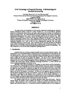
Nevertheless, the combination of a nature-inspired algorithm with a deterministic method to deal with large exponents has been reported as a competitive approach. This is the case of the sliding window method (SWM) and the artificial immune system (AIS) in (Cruz-Cort´es et al., 2008). The sliding window method (SWM) uses the binary representation of the exponent e, e = (em−1 em−2 . . . e1 e0 ), which is divided in zero and non-zero windows or words of variable length. The partitioning process is shown in Figure 4.

Figure 4: Process to generate zero and non-zero windows

The complete pseudocode of the SWM is presented in Algorithm 7. In the first version of SWM, the step 2 of the algorithm required only a sequence of integer numbers from 1 to 2k − 1, where k is the maximum size of a window. However an improved version proposed in (Bos and Coster, 1990) considered the usage of addition sequences instead of the simple sequence of numbers. This improved version, as indicated in Algorithm 7, is used in this work. An addition sequence for a set of given numbers [n0 , n1 , . . . , nm ] is a list of numbers that satisfies the properties of an addition chain, with the particularity that the given numbers occur in such sequence (Bos and Coster, 1990). For example, for the next sets of numbers: [13, 35, 89, 97] a possible addition sequence can be; [1, 2, 3, 5, 8, 13, 16, 19, 35, 54, 89, 97]. 24

Algorithm 7 Sliding Window Method using addition sequences Require: Integer e = (em−1 . . . e1 e0 ) Ensure: Addition Chain U = (1, 2, . . . , e) 1: Decompose e into h zero and non-zero windows Wi 2: Generate an addition sequence corresponding to the N Z windows [W0 , W1 , . . . , WN Z−1 ] 3: Add addition sequence to end list U 4: Set x = Wh−1 5: for i = eh−2 to e0 do 6: x=2∗x 7: Add x to end list U 8: if ei == last bit of current N Z window then 9: x = x+ decimal value of the current N Z window 10: Add x to end list U 11: end if 12: end for 13: return U

Besides traditional methods to generate addition sequences as the one detailed in Algorithm 8, the AIS algorithm has been used to find minimal length addition sequences (Cruz-Cort´es et al., 2008). This is then the way the deterministic method is combined with the stochastic one: SWM focuses on finding minimal length ACs while the AIS helps by providing SWM with minimal length addition sequences. Algorithm 8 Addition sequence generator Require: A sorted set of n integers U = e1 , e2 , . . . en−1 , en in ascending order. Ensure: Addition sequence e1 , e2 , . . . en−1 , en . 1: k = n − 2 2: Set U = u1 = e1 , u2 = e2 , . . . , uk = en−2 3: H = h1 = en−1 , h2 = en 4: W = ø 5: while U 6= ø do 6: ∆ = (h2 − h1 ) 7: W = W ∪ h2 8: h1 , h2 = max two elements(uk , ∆, h1 ) 9: if ∆ < uk and ∆ ∈ / U then 10: U = sortSet(U ∪ ∆) 11: end if 12: if ∆ ∈ U then 13: k =k−1 14: end if 15: end while 16: return W

In this work ACEP is coupled in a similar way to SWM (ACEP-SWM) as detailed in Algorithm 9, where max M SW is the maximum size of the Most Significant Window (MSW) which is always the first window (Cruz-Cort´es et al., 2008) and q is the maximum number of consecutive zeros allowed 25

to make non-zero windows. The work of the stochastic method (ACEP in this case), is to generate a minimal length addition chain U for the decimal number representing the first non-zero window (Step 5 in Algorithm 9). An element from U will be then chosen (step 6 in Algorithm 9) and combined with the decimal values of the remaining windows (step 7 in Algorithm 9) so as to generate an addition sequence with Algorithm 8 (step 8 in Algorithm 9). This sequence will be mixed with U to generate the final addition sequence to be used by the sliding window method (step 9 in Algorithm 9). Algorithm 9 ACEP for Addition sequences Require: Integer e = (em−1 . . . e1 e0 ) , max M SW, q Ensure: Addition Sequence Seq = (1, 2, . . . , m) 1: Decompose e into h zero and non-zero windows Wi using max M SW bits for the most significant window (MSW) and a maximun of q consecutive zeros to make non-zero windows 2: Represent in decimal the non-zero windows 3: Set M SW = W0 4: Sort non-zero windows in ascending order List = {W0 , W1 , . . . , WN Z−1 } 5: Set U = ACEP(M SW ) 6: Select a suitable element a ∈ U such that a > WN Z−2 7: Set List = {W0 , W1 , WN Z−1 , a} 8: Set List = Addition sequences generator (List) 9: Set Seq = List + U The following experiment compares the best results obtained by ACEPSWM, AIS-SWM (Cruz-Cort´es et al., 2008) (i.e. the same Algorithm 9 but using AIS instead of ACEP in step 5) and the SWM with the traditional addition sequence generator(Kaya-Koc, 1994) (Algorithms 7 and 8), in ten random exponents e with large bit-length m = 128, 256, 512 and 1024. The parameters values used by ACEP are the same adopted in experiment 1 (with 92,000 evaluations). A comparison based on the best results found out of 30 independent runs per exponent is presented in Table 9, where k is the window size required by SWM. Based on the results both, AIS-SWM and ACEP-SWM, outperformed SWM with the traditional addition sequence generator. Regarding the two methods based on a nature-inspired algorithm, AIS-SWM provided slightly better results with m= 128 with respect to ACEP-SWM. However, ACEP26

m 128 256 512 1024

SWM length 156 308 607 1195

k 4 4 5 5

AIS-SWM length MSW 153 17 304 13 604 11 1196 6

q 2 2 2 5

ACEP-SWM length MSW 154 8 304 6 604 17 1190 14

q 2 2 2 2

Table 9: Best ACs found by ACEP-SWM, AIS-SWM (Cruz-Cort´es et al., 2008) and the SWM with the traditional addition sequence generator (Kaya-Koc, 1994) in large exponents. A result in boldface means a better result

SWM outperformed AIS-SWM with the largest exponent tested (m=1024). In the two remaining m values (256 and 512) similar results were found by both algorithms. 6. Conclusions and future work An adapted evolutionary programming algorithm to find minimal length addition chains (ACEP) was introduced in this paper. The adaptations consisted on (1) a suitable solution representation at the phenotype level (i.e., not encoded) and a simple fitness function based on the length of each solution, (2) a mechanism to generate a complete feasible initial population (i.e. only feasible addition chains were generated), (3) a special mutation operator to generate new feasible solutions and (4) a replacement mechanism based on stochastic encounters to avoid premature convergence. ACEP was tested in three experiments with different types of exponents: small, hard, and diverse. In the fourth experiment ACEP was used to generate Euclidean addition chains in the set of diverse exponents. Furthermore, ACEP was coupled with the deterministic method called sliding window method (SWM) to solve large exponents; ACEP was in charge of helping on the generation of minimal length addition sequences while SWM used such sequences to generate minimal length addition chains. In the first experiment ACEP outperformed the compared algorithms in four, out of six, sets of “small” exponents by requiring only 92,000 evaluations with respect to the 240,000 and 350,000 required by the other approaches. Furthermore, ACEP outperformed all algorithms in the six sets of exponents by performing 240,000 evaluations. In the second experiment, ACEP obtained similar results as those obtained with the GA but requiring only 38% 27

of the evaluations performed by such approach. In the third experiment, ACEP obtained similar results in all but one diverse exponents by using only 8% of the evaluations required by PSO. Furthermore, in one exponent ACEP improved the results reported by the compared approaches (PSO and AIS). The fourth experiment showed the capabilities of ACEP to deal with Euclidean addition chains on the set of diverse exponents. Finally, in the fifth experiment, the combination of ACEP-SWM solved a set of large exponents where the shortest addition chains for the largest exponent were generated by ACEP. From the overall results it can be seen that ACEP covered a wide set of exponents with respect to other nature-inspired-based approaches to find minimal length addition chains. Furthermore, its computational cost, measured by the number of evaluations computed (a well-accepted measure in the evolutionary computing literature), is significantly lower with respect to the compared approaches. Finally, ACEP is easy to implement. The future work consists of further tests of ACEP in Euclidean addition chains and a study of their parameter values. Finally ACEP will be implemented in a public-key encryption system, such as RSA or DSA with the goal of measuring its performance. Acknowledgements The first author acknowledges support from the Mexican Council for Science and Technology (CONACyT) through a scholarship to pursue PhD studies at the University of Veracruz. References Bola˜ nos, F., Bernal, A., 2008. A hardware optimized implementation for the modular exponentiation operator. Dyna 75, 55–63. Bos, J., Coster, M., 1990. Addition chains heuristics, in: Advanced in Cryptology. Proceedings of CRYPTO’89, Springer-Verlag. pp. 400–407. Cruz-Cort´es, N., Rodr´ıguez-Henr´ıquez, F., Coello-Coello, C.A., 2008. An artificial immune system heuristic for generating short addition chains. IEEE Transactions on Evolutionary Computation 12, 1–24.

28

Cruz-Cort´es, N., Rodr´ıguez-Henr´ıquez, F., Ju´arez-Morales, R., CoelloCoello, C.A., 2005. Finding optimal addition chains using a genetic algorithm approach, in: Proceedings of the Computational Intelligence and Security Conference (CIS’2005), Springer-Verlag. pp. 208–215. Dorigo, M., Maniezzo, V., Colorni, A., 1996. The Ant System: Optimization by a Colony of Cooperating Agents. IEEE Transactions of Systems, Man and Cybernetics-Part B 26, 29–41. ElGamal, T., 1985. A public key cryptosystem and a signature scheme based on discrete logarithms. IEEE Transactions on Information Theory 31, 469–472. Fogel, L.J., 1999. Intelligence Through Simulated Evolution. Forty years of Evolutionary Programming. John Wiley & Sons, New York. Fumaroli, G., Vigilant, D., 2006. Blinded fault resistant exponentiation, in: Breveglieri, L., et. al (Eds.), Proceedings of the Workshop on Fault Diagnosis and Tolerance in Cryptography (FDTC’2006). Springer-Verlag. volume 4236 of Lecture Notes in Computer Science, pp. 62–70. Herbaut, F., Liardet, P.Y., Mloni, N., Tglia, Y., Vron, P., 2010. Random euclidean addition chain generation and its application to point multiplication, in: Gong, G., Gupta, K. (Eds.), Progress in Cryptology - INDOCRYPT 2010. Springer Berlin Heidelberg. volume 6498 of Lecture Notes in Computer Science, pp. 238–261. Joye, M., 2009. Protecting RSA against fault attacks: The embedding method, in: Proceedings of the Workshop on Fault Diagnosis and Tolerance in Cryptography (FDTC’2009), IEEE Computer Society, Los Alamitos, CA, USA. pp. 41–45. Kaya-Koc, C., 1994. High-Speed RSA Implementation. Technical Report TR 201. RSA Laboratories, Redwood City, CA. Knuth, D.E., 1981. The art of computer programing. 2nd ed., AddisionWesley. Kunihiro, N., Yamamoto, H., 1998. Window and extended window methods for addition chain and addition-subtraction chain. IEICE Transactions

29

on Fundamentals of Electronics, Communications and Computer Sciences E81-A, 72–81. Lawson, N., 2009. Side-channel attacks on cryptographic software. IEEE Security and Privacy 7, 65–68. Le´on-Javier, A., Cruz-Cort´es, N., Moreno-Armend´ariz, M.A., OrantesJim´enez, S., 2009. Finding minimal addition chains with a particle swarm optimization algorithm, in: Proceedings of the Mexican International Conference on Artificial Intelligence (MICAI’2009), pp. 680–691. Nedjah, N., de Macedo-Mourelle, L., 2006. Towards minimal addition chains using ant colony optimisation. Journal of Mathematical Modeling and Algorithms 5, 525–543. Nunes de Castro, L., Timmis, J., 2002. Artificial Immune Systems: A New Computational Intelligence Approach. Springer Verlag. Osorio-Hern´andez, L.G., Mezura-Montes, E., Cruz-Cort´es, N., Rodr´ıguezHenr´ıquez, F., 2009. An improved genetic algorithm able to find minimal lenght addition chains for small exponents, in: Proceedings of the IEEE Congress on Evolutionary Computation, IEEE Press. pp. 1422–1429. Quisquater, J.J., Koene, F., 2002. Side channel attacks: State of the art. Technical Report. Information-Technology Promotion Agency. Japan. Rivest, R.L., Shamir, A., Adleman, L., 1978. A method for obtaining digital signatures and public-key cryptosystems. Communications of the ACM 21, 120–126. Rodriguez-Cristerna, A., Torres-Jimenez, J., 2013. A genetic algorithm for the problem of minimal brauer chains for large exponents, in: Melin, P., Castillo, O. (Eds.), Soft Computing Applications in Optimization, Control, and Recognition. Springer Berlin Heidelberg. volume 294 of Studies in Fuzziness and Soft Computing, pp. 27–51. Ryabko, B., Fionov, A., 2005. Basics of Contemporary Cryptography for IT Practitioners. volume 1 of Series on Coding Theory and Cryptology. World Scientific.

30

Van-Der Kruijssen, S., 2007. Addition Chains, efficient computing of powers. Bachelor’s Thesis. University of Amsterdan. Amsterdan. Wu, C.L., Lou, D.C., Lai, J.C., Chang, T.J., 2006. Fast exponentiation algorithm for RSA public-key cryptosystems. Informatica 17, 445–462.

31