AIAA Paper AIAA-2006-6955, 11th AIAA/ISSMO Multidisciplinary Analysis and Optimization Conference, Portsmouth, VA, September 6-8, 2006.
Evolutionary Wavelet Neural Network for Large Scale Function Estimation in Optimization Debasis Sahoo1 and George S. Dulikravich2 Department of Mechanical and Materials Engineering Multidisciplinary Analysis, Inverse Design, and Robust Optimization Center (MAIDROC) Florida International University, 10555 W. Flagler St., Miami, Florida 33174, U.S.A. e-mail:
[email protected] Web page: http://maidroc.fiu.edu
This paper describes a new method for constructing wavelet neural network in order to improve the accuracy of prediction for multi-dimensional function spaces. An algorithm is developed using the concept of evolutionary search in wavelet neural network. It helps in decreasing the computational effort needed for building the wavelet neural network. Several modifications to wavelet neural network are also suggested for improving its performance in predicting non-linear function spaces. These algorithms were tested using diverse test functions. These networks can be effectively used as non-linear system estimators for large scale optimization problems.
I. Introduction Function estimation involves finding the underlying relationship from a given set of input-output dataset. This has been popular in various applications such as pattern classification, data mining, system identification, and response surface construction in optimization1,2,3. The system identification problem is to estimate the underlying system characteristics using a set of empirical input-output data. Recently, feed-foreword neural networks such as multilayer perceptron (MLP) and radial basis function networks (RBFN) have been widely used as an alternative approach to function approximation. They provide a generic black box function representation and have been shown to be capable of approximating any continuous function defined on a compact set of data with arbitrary accuracy2. Using the concept of locally supported basis function, such as RBFN, a class of wavelet neural network (WNN) has become popular lately3-7. It also uses the concept of wavelet decomposition. Combining wavelet and neural networks diminishes the weakness of each other7. The resulting network is capable of handling problems of moderately large dimension and can be efficiently constructed. Due to the radial structure of the wavelets, it can be considered as a more general form of RBFN. Few modifications to such networks were suggested to deal with outliners in training data8. This helps in training the WNN with noisy dataset. Constructing WNN involves estimating the parameters in the nodes of the network and the weights. This is done by minimizing a cost function which reflects the approximation quality of the network7,9. Such networks can be used to predict non-linear function spaces in optimization. Several methods to build a surrogate model for similar purpose in optimization have been tried by Dulikravich et al.10-12. Applications like response surface construction for multi-objective optimization require an estimating function having large number of design variables. Building WNN for such functions is computationally expensive. So, instead of preparing a huge library of wavelets7 an evolutionary based search algorithm is suggested for large dimensional function estimation. In this paper, we propose a genetic algorithm (GA) search for setting the network parameters in a WNN. Several modifications to the basis function and network architecture are also studied. The networks so created were tested using many well known test functions to validate their accuracy and robustness. Finally, we present a hybrid wavelet neural network capable of estimating highly non-linear function spaces with good accuracy and using lesser computational resources. 1 2
Graduate student. Student member AIAA. Professor and Chairman of the Department. Director of MAIDROC. Associate Fellow AIAA.
1 American Institute of Aeronautics and Astronautics
II. Genetic Algorithm based Wavelet Neural Network
Wavelets occur in the family of functions generated from a mother wavelet ψ ( x ) . Each wavelet in it is defined by dilation vector
ai which controls the scaling and translation vector t i which controls the position. Given a
training set, the overall response of a WNN can be arithmetically written as p ⎛ x −t ⎞ f ( x ) = w0 + ∑ wiψ i ⎜ ⎟ ⎝ a ⎠ i =1
N
where N p is the number of wavelet nodes in the hidden layer and
(1)
wi is the synaptic weight for each hidden node in
the WNN. The dilation and translation vectors have size equals to the number of variables in the estimated function. Such a network can be used to approximate any function.
y = f (x ) + ε where
(2)
f is a regression function and the error term ε is a zero-mean random variable of disturbance.
One of the well known approaches for constructing WNN7 requires the generation of a wavelet library, W . This library is composed of discretely dilated and translated versions of mother wavelet function ψ ( x ) . The next step is selecting the best wavelets based on the training data from this library to build the regression. This approach for building WNN becomes computationally expensive when the estimated function has a huge number of variables. This is due to exponential increase of the size of the wavelet library W with the dimension of the estimated function. Searching such a huge library one-by-one is computationally redundant. Therefore, the stochastic approach for searching the best wavelets for the WNN hidden nodes is proposed. The concept of binary GA was used to search for the wavelets required for the hidden nodes in the WNN. The dilation and translation factors (binary representation) for each dimension of the wavelet were concatenated to form the chromosomes in the GA population. A typical representation of a wavelet in 2-D function estimation looks like
1
t1 0 1 1
1
a1 1 1 1
1
t2 1 0 1
0
a2 0 0 1
Figure 1. Binary string representation of a 2-D wavelet. It has two dilatation factors specifying the scaling and two translation factors specifying the position of the wavelet in each dimension. The variables space is normalized so the translation factors can vary within [-1, 1] and the dilation factors were varied within [0.1, 0.8]. The fitness for selecting the wavelet was defined as the norm of the residue obtained by doing Multiple Linear Regression (MLR) of the values given by the wavelet transform of the training data vs. the real function values. The GA was run for a sufficient number of generations to select a wavelet. Subsequent wavelets were searched by the GA based on the residue obtained in former step set as target values. This approach was unable to search for proper wavelets when the number of variables in the estimated function went beyond ten. The chromosome length for such functions was huge and the binary GA became inefficient. Therefore, a real numbers GA based search was proposed. In real numbers GA, the wavelet is represented as a string of real number instead of a binary string. The range for searching for the values of dilation factors was relaxed to [0.005, 5.00]. This gave more flexibility to the GA for searching appropriate wavelets. A typical example of a wavelet representation in 4-D function estimation is a1 2.8424
t1 0.25483
a2 2.4672
t2 0.000922
a3 1.7407
t3 0.98521
a4 2.5848
t4 -0.61214
Figure 2. Real string representation of a 4-D wavelet. The fitness assignment was similar to the previous method. In addition, Whole Arithmetic Crossover and Floating Point Mutation operators were used13. Separate GAs were run serially for finding the activation function in each node of the WNN architecture.
2 American Institute of Aeronautics and Astronautics
III. Modifications to Basis Function and Architecture Training the WNN for response surface generation was done using a random dataset. The size of the dataset required to reach a given accuracy can be decreased by using Sobol Quasi-Random Sequence14 instead of random training data. Sobol sequence scatters points in the n-dimensional space uniformly. WNN trained on such a distribution learns the function space uniformly. This helps in reducing the computational effort needed in training a WNN to achieve a given accuracy. Typically, the mother wavelet used in the WNN is Mexican Hat wavelet described by the following function.
⎛ 2
ψ ( x ) = ⎜⎜
⎝ 3
⎛ − x2 ⎞ ⎟⎟ ⎝ 2 ⎠
⎞
π −1 / 4 ⎟⎟(1 − x 2 )exp⎜⎜ ⎠
(3)
Gaussian wavelets were used with this mother wavelet to construct the WNN. For each node of the WNN, GA searched the best Mexican Hat wavelet as well as the best Gaussian Wavelet. The one having a lower norm of residue after performing MLR was selected and inserted in the WNN architecture. The overall architecture of WNN had a mixture of Mexican Hat and Gaussian wavelets and looked like:
Figure 3. Mixed architecture of WNN using Mexican Hat and Gaussian wavelets To improve the accuracy of prediction further few other parameters were introduced with dilation and translation vectors. An exponent parameter, n , which controlled the sharpness of the basis function was used. The mapping of the input variable for the mother wavelet so obtained can be expressed as
⎛ x−t ⎞ x=⎜ ⎟ ⎝ a ⎠
n
(4)
Now the GA string had three parameters per each dimension of the function. The limits for the exponent parameter was set within [0.9, 1.2] and produced more accurate predictions. The following figures show the impact of the exponent parameter on the shape of the basis function used in the WNN. Another parameter to control the skewness was introduced in the basis function. This parameter, p , controlled the magnitude and direction of skewness of the basis function. Following is the mathematical description of a skewed Gaussian distribution.
⎛ − x2 ⎞ ⎛ 2 −1 / 4 ⎞ ⎟⎟ * X ( P.5 ) ψ (x ) = ⎜⎜ π ⎟⎟ exp⎜⎜ ⎝ 3 ⎠ ⎝ 2 ⎠
(
)
(5)
The parameter p can take only integral values and the magnitude of skewness is governed by its absolute value. The direction of skewness is governed by the vector X in the governing equation.
3 American Institute of Aeronautics and Astronautics
Figure 4. Shape of Gaussian basis function with exponent parameter n = 0.8 and n = 2.0
Figure 5. Plan view of skewed wavelets: (a) negative x-axis (b) negative x-axis and positive y-axis. Plan views of 2-D skewed wavelets are shown above. It shows that the wavelet basis function can also be skewed in multiple directions simultaneously. The value of parameter p was set between [-5, 5] to determine the proper wavelet for the WNN nodes. All these parameters (a, t, n, and p) for each dimension of the wavelet were searched using real based GA.
Figure 6. Hybrid WNN architecture using full training dataset.
4 American Institute of Aeronautics and Astronautics
This network showed superior performance for a large variety of test problems. The accuracy of highly nonlinear function estimation was still a problem. To improve it further the concept of using multiple WNN in a single architecture was proposed. This idea can be implemented in two different ways. First, the training dataset can be divided into a fixed number of exclusive sets and each of these can be used to train a network separately. Second, multiple networks can be created by training each of them with the complete training dataset available. After generating all the trained sub-networks the hybrid WNN was created assembling each one of them to form a single network with proper weights. After a few tests, the idea of training each sub-network with a complete training dataset was concluded to give better accuracy. Here, the number of sub-networks ‘S’, needed in the final architecture was decided in advance. The full dataset was used to train s-WNNs separately and generate suitable sub-networks. Once all the sub-networks are created, the full training data is used to obtain the weights for each of them. Linear regression of the output of each of these networks with the target value is done in order to obtain the weights.
IV. Test Functions and Testing Scheme For testing different versions of WNN prepared here several mathematical test functions were developed. The dimension of test functions varied from 2 – 7. This would help to evaluate the performance of each of them vs. the dimension of the estimated function. These test functions were developed using many elementary functions for studying the robustness of WNN. The test functions so developed are tabulated below: Table 1 Test functions developed using elementary functions Dimension of Function 7D
Function Used for Testing
1 + x 1 + x 3 ⋅ sin(x 2 ) + exp(x 3 ) ⋅ cos(x 4 ) - log(2 + x 5 ) ⋅ (x 6 + 7) ⋅ (x 37 )
6D
1 + x 1 + x 3 ⋅ sin(x 2 ) + exp(x 3 ) ⋅ cos(x 4 ) - log(2 + x 5 ) ⋅ (x 6 + 7) ⋅ (x 34 )
5D
1 + x 1 + x 3 ⋅ sin(x 2 ) + exp(x 3 ) ⋅ cos(x 4 ) - log(2 + x 5 ) ⋅ (x 3 + 7) ⋅ (x 34 )
4D
1 + x 1 + x 3 ⋅ sin(x 2 ) + exp(x 3 ) ⋅ cos(x 4 ) - log(2 + x 2 ) ⋅ (x 3 + 7) ⋅ (x 34 )
3D
1 + x 1 + x 3 ⋅ sin(x 2 ) + exp(x 3 ) ⋅ cos(x 2 ) - log(2 + x 2 ) ⋅ (x 3 + 7) ⋅ (x 13 )
2D
1 + x 1 + x 1 ⋅ sin(x 2 ) + exp(x 2 ) ⋅ cos(x1 ) - log(2 + x 2 ) ⋅ (x 1 + 7) ⋅ (x 13 )
WNNs were trained using 40 Sobol points and were tested using 30 subsequent Sobol points. All the networks had about 8 – 12 nodes in the hidden layer of the NN. The tested points were divided into six groups depending on the amount of error for assessment. Finally, for each of these test functions stacked bar plots of percentage of tested points falling in each group was made in order to compare them. Table 2 Groups for dividing tested data for evaluation Group Number Error Value
1 0-10%
2 10-20%
3 20-50%
4 50-100%
5 100-200%
6 >200%
The above testing scheme was used to evaluate the performance of several versions of WNN suggested. Later, few well known test functions15 were used to evaluate the performance of WNN having different basis functions and hybrid WNN was also tested. Chen et al. gave metrics to evaluate the performance of prediction. Most of the test problems had typical features of engineering problems. Two relative scales were considered (number of variables ≥ 10 and number of variables = 2, 3). Both low-order nonlinear as well as high-order nonlinear problems were used. And finally, one test problem had noisy behavior. All the test problems obtained were selected from the book by Hock and Schittkowski16 which offers many other problems for testing nonlinear algorithms. Second order polynomial models have k = (n + 1)(n + 2) / 2 coefficients for n design variables. Kaufman et 17 al. found that 1.5k sample points for 5-10 variable problems and 4.5k sample points for 20-30 variable problems were necessary to obtain reasonably accurate second order polynomial models. Therefore, for small scale problems (number of variables = 2, 3), 10 n data points were used. For large scale problems (number of variables > 10), 3k data points were used to train the WNN. For testing each model, 1000 – 1200 Sobol points were used.
5 American Institute of Aeronautics and Astronautics
The performance of any technique to predict functional space can be measured in various aspects like robustness, efficiency, transparency, and conceptual simplicity. To assess the accuracy of the WNN three different metrics were used: R Square, relative average absolute error, and relative maximum absolute error. The equations for these three metrics are given below: R Square: n
R2 = 1−
∑ (y i =1 n
∑ (y i =1
Here,
2 − yˆ i )
i
i
− y)
= 1−
2
MSE variance
(6)
yi is the observed value, yˆ i is the predicted value, and y is the mean of observed value. MSE (Mean Square
Error) represents the departure of the model from the real simulation model, and the variance captures the magnitude of irregularity in the problem. The larger the value of R Square, the more accurate the model is. Relative Average Absolute Error (RAAE): n
RAAE =
∑
i =1
y i − yˆ i (7)
n ∗ STD
Here STD stands for the standard deviation. The smaller the value of RAAE, the more accurate the model is. This is usually highly correlated with R Square. Relative Maximum Absolute Error (RMAE)
RMAE =
max ( y1 − yˆ 1 , y 2 − yˆ 2 ,..., y n − yˆ n
)
STD
(8)
Large RMAE indicated large error in one region of the design space even though the overall accuracy indicated by R Square and RAAE can be very good. This metric cannot show the overall performance in the design space, so it is not as important as the other two. Based on the above scheme, different real parameter GA based WNN were tested. The magnitude of the metrics showed the accuracy of the model and the variance of the metrics values among different problems illustrates the robustness of the model.
V. Results of Various Test Functions The test results for a different version of WNN developed are shown in this section and its performance is analyzed. First, the impact of using Sobol sequence instead of random training data on the efficiency of WNN was studied. For this study a 2-D test function was designed and used to evaluate the performance of WNN trained on Sobol sequence vs. WNN trained on random training data. The mathematical expression describing the test function is:
(
)
y = x12 − x 2 ⋅ sin (5 x1 ) ⋅ sin (6 x 2 )
(9)
The training of WNN using random data required 400 points. Similar accuracy on training data could be achieved using only 100 Sobol points to train the second WNN. The required accuracy of 10% error on training data was achieved in 18.37 seconds using random data points where as the WNN trained with Sobol14 data points took only 8.56 seconds. The following plots show the real function space and the estimated function space using Sobol points for training. Studying the residue of estimated function vs. the number of nodes in the WNN we concluded that the WNN trained with Sobol points reached lower residue faster than the WNN trained with random points. Therefore, training the WNN using Sobol points helped to build models faster and more accurately.
6 American Institute of Aeronautics and Astronautics
Figure 7. (a) The real 2-D function space (b) The estimated function space using Sobol trained WNN. Accuracy of binary GA based WNN and real GA based WNN in predicting function spaces were studied using a set of test functions [Table 1]. Following stacked bar plots shows the percentage of testing data points having particular ranges of error for several test functions. Real GA Based WNN
Real GA Based WNN 100% Percentage of Testing Data Points in Each Group
Percentage of Testing Data Points in Each Group
100% 90% 80% 70%
>200%
60%
100-200% 50-100%
50%
20-50%
40%
10-20%
30%
0-10%
20% 10% 0%
90% 80% 70%
>200%
60%
100-200% 50-100%
50%
20-50%
40%
10-20%
30%
0-10%
20% 10% 0%
2D
3D
4D
5D
6D
7D
2D
Dim ension of Test Function
3D
4D
5D
6D
7D
Dim ension of Test Function
Figure 8. Stacked bar plots of percentage of tested data having specific error: (left) binary GA based WNN, (right) real GA based WNN It shows that the percentage of data having good prediction (0 – 10 % error) decreases as the dimension of function increases. Real GA based WNN out performs binary GA based WNN in all of the test function and is chosen for future model preparation. The effect of dimension of the function on the computational expense required for training the WNN was analyzed. It showed that the time taken to train a single WNN using a single processor varied linearly with the dimension of the function. CPU Time Taken to Construct the WNN 250
CPU Time (Seconds)
200
150
100
50
0 2D
3D
4D
5D
6D
7D
Dim ension of Tested Function
Figure 9. Computing time required by a single processor for building WNN for various test functions.
7 American Institute of Aeronautics and Astronautics
The accuracy of predictions for the same test functions were improved further by adding the concept of mixed architecture along with the exponent parameter ‘p’. The following stacked bar plot shows the improvement for each of the test functions.
100% 90% 80% 70%
>200% 100-200%
60%
50-100%
50%
20-50%
40%
10-20% 0-10%
30% 20% 10%
7D -OLD
7D - NEW
6D - OLD
6D - NEW
5D - OLD
5D - NEW
4D - OLD
4D - NEW
3D - OLD
3D - NEW
2D - OLD
0% 2D - NEW
Percentage of Testing Data Points in Each Group
Real GA Based WNN: Addition of Exponent Term
Dimension of Test Function
Figure 10. Improvement in accuracy of WNN using mixed architecture and exponent parameter. This extra parameter helped in finding a more accurate description of the estimated function locally. The GA searches for the proper set of parameters to construct the WNN efficiently. The current version of WNN was further tested using thirteen test problems provided by Chen et al.15. The performance metrics were compared to evaluate the performance of WNN in predicting various functions. The value of R-Square shows the average accuracy of prediction and was used primarily for performance evaluation. R-Square value of one is produced when the predictions are 100% accurate and a value of zero shows random predictions. The following plot shows the value of R-Square for each of the test functions given by WNN when prepared using three different types of basis functions: Gaussian, Mexican Hat and Skewed Gaussian (Chi-Square). The values of R-Square for most of the test problems using Gaussian and Mexican Hat wavelet approaches one. Thus, such basis functions were suitable for building accurate models. Few problems (1, 3, 9, and 10) had lower values of R-Square and implied that the WNN was unable to predict these with good accuracy. These problems were highly non-linear. WNN was able to predict problem number 13 with good accuracy, though the problem had a lot of noise. To improve the WNN to predict highly non linear functions more accurately, hybrid WNN were used. Two hybrid WNNs were prepared and tested using the same 13 test problems. One of them had sub-networks trained using exclusive sets of the whole training dataset and the other had sub-networks trained on the full training dataset. The results were compared with the predictions using single Mexican Hat WNN. Clear improvements in predictions were seen using hybrid WNN having sub-networks trained on full training dataset. Hybrid WNN with sub-networks trained on excusive sets of training data did predict better then single WNN (problem number 6 and 10) but had worse predictions (problem number 1 and 3) also. Therefore, hybrid WNN with sub-networks trained on full training dataset was suggested for highly non-linear function spaces. About 5 – 6 sub-networks are recommended in the architecture of hybrid WNN. Finally, the performance of the single network WNN vs. the dimension of estimated function was studied. Problem number 2 was chosen15 and the number of variables was varied to get several test functions. WNN was trained on 400 Sobol points and the model was confirmed using 1200 testing points. The accuracy of predictions and the computational expense was compared among these test functions. The following plot compares the R-Square values and the time taken by a single processor to generate the model for the test functions having different number of dependent variables.
8 American Institute of Aeronautics and Astronautics
Comparison of R Square for various wavelets used Gaussian Wavelet
1.2
Mexican Hat Wavelet ChiSQ Wavelet (Skewed)
1
R Square
0.8
0.6
0.4
0.2
0 PB1
PB2
PB3
PB4
PB5
PB6
PB7
PB8
PB9
PB10
PB11
PB12
PB13
Problem Number
Figure 11. R-square values for test functions obtained using different basis functions.
Mexican Hat Wavelet Comparison of R Square for various wavelets used
Hybrid WNN(EXCLUSIVE) Hybrid WNN(FULL TRAINING)
1 0.9 0.8 0.7 R Square
0.6 0.5 0.4 0.3 0.2 0.1 0 PB1
PB2
PB3
PB4
PB5
PB6
PB7
PB8
PB9
PB10
PB11
PB12
PB13
Problem Number
Figure 12. R-square values for test functions using various hybrid WNN. Figure 13 shows that the accuracy of the model prediction decreases as the number of design variables increases. One reason for this is the constant number of training points used to build each WNN. Also, the time taken by a single processor to build various WNN models goes on increasing with the dimension of the estimated functions. The GA takes longer to search for the proper nodes as the dimension of the function increases. Assuming the value of R Square > 0.5 is good prediction, one can predict function having 90 variables effectively (extrapolating). Thus, this algorithm can predict high dimensional function space, but the level of function non-linearity is always a factor governing the accuracy of prediction.
9 American Institute of Aeronautics and Astronautics
RSQ CPU Time
1.2
1400.00 1200.00
1
1000.00 800.00 0.6 600.00
CPU time
R Square
0.8
0.4 400.00 0.2
200.00
0
0.00 10
20
30
40
# of variables
Figure 13. Variation of accuracy and computational expense with dimension of test function.
VI. Conclusions This paper presents a novel technique to search the proper activation functions for the construction of WNN. Such a method helps to build response surface for predicting high dimensional function spaces accurately and efficiently. Several modifications to the architecture and basis function in WNN were suggested and tested using diverse test functions. Simulation results show that WNN for predicting function having large number of variables (~90) can be implemented accurately. The modified WNN developed in such a way had about 5 – 7 % average absolute error on training data in most of the test problems. The final testing for most of the test functions was done using 1000 – 1200 data points. With such large testing dataset we can assume that any further prediction of the functional space will have similar accuracy. It was found that about ten to twelve activation nodes in the hidden layer of WNN were adequate for good predictions i.e. 5% average absolute error on training data. Further addition of activation nodes in WNN improved the accuracy on training data only slightly, but did not help in improving the accuracy on testing data further. This implies that for the given dataset a WNN with about ten to twelve activation nodes extracted most of the information regarding the topology of the functional space. Finally, a hybrid WNN network was developed using the concept of having multiple WNNs and helped in increasing the accuracy of prediction of highly non-linear functional spaces.
Acknowledgement The authors are grateful for the financial support provided for this work by the US Air Force Office of Scientific Research grant FA9550-06-1-0170 monitored by Dr. Todd E. Combs and by the US Army Research Office/Materials Directorate under the contract number DAAD 19-02-1-0363 monitored by Dr. William M. Mullins.
References 1
Chen, D. S. and Jain, R. C., “A Robust Back Propagation Learning Algorithm for Function Approximation”, IEEE Trans. Neural Networks, Vol. 5, May 1994, pp. 467 – 479. 2 Hwang, J.N., “Nonparametric Multivariate Density Estimation: A Comparative Study,” IEEE Trans. Signal Processing, Vol. 42, 1994, pp. 2795-2810. 3 Shashidhara, H. L., Lohani, S. and Gadre, V. M., “Function Learning using Wavelet Neural Networks,” Proceedings of IEEE International Conference on Industrial Technology, Vol. 2, 2000, pp. 335-340. 4 Cristea, P., Tuduce, R. and Cristea, A., “Time Series Prediction with Wavelet Neural Networks,” In Proceedings of the 5th seminar on IEEE Neural Network Applications in Electrical Engineering, 2000. pp. 5-10. 5 Ho, D. W. C., Zhang; P.-A. and Xu, J., “Fuzzy Wavelet Networks for Function Learning,” IEEE Transactions on Fuzzy Systems, Vol. 9, No. 1, Feb 2001, pp. 200-211. 6 Zhang, J., Walter, G. G. Miao, Y. and Lee, W. N. W., “Wavelet Neural Networks for Function Learning,” IEEE Trans. Signal Processing, Vol. 43, June 1995, pp. 1485-1497. 7 Zhang, Q., ”Using Wavelet Network in Nonparametric Estimation”, IEEE Trans. Neural Network, Vol. 8, 1997, pp.227-236.
10 American Institute of Aeronautics and Astronautics
8
Li, S. T. and Chen, S. C., “Function Approximation using Robust Wavelet Neural Network", Proceedings of the 14th IEEE International Conference On Tools with Artificial Intelligence (ICTAI 2002), Washington D.C., November 4-6, 2002, pp. 483-488. 9 Zang, Q. and Benveniste, A., “Wavelet Networks,” IEEE Transactions on Neural Networks, Vol. 3, No. 6, November 1992. 10 Dulikravich, G. S. and Egorov, I. N., “Robust Optimization of Concentrations of Alloying Elements in Steel for Maximum Temperature, Strength, Time-To-Rupture and Minimum Cost and Weight,” ECCOMAS – Computational Methods for Coupled Problems in Science and Engineering, Fira, Santorini Island, Greece, May 2528, 2005. 11 Dulikravich, G. S. and Egorov, I. N., “Optimization of Alloy Chemistry for Maximum Stress and Time-toRupture at High Temperature,” AIAA paper 2004-4348, 10th AIAA/ISSMO Multidisciplinary Analysis and Optimization Conference, eds: A. Messac and J. Renaud, Albany, NY, Aug. 30 – Sept. 1, 2004. 12 Egorov-Yegorov, I. N. and Dulikravich, G. S., “Chemical Composition Design of Superalloys for Maximum Stress, Temperature and Time-to-Rupture Using Self-Adapting Response Surface Optimization”, Materials and Manufacturing Processes, Vol. 20, No. 3, May 2005, pp. 569-590. 13 Wright, A. H., “Genetic Algorithms for Real Parameter Optimization”. In G. J. E. Rawlins (Ed.), Foundations of Genetic Algorithms, 1991, pp. 205-218. 14 Sobol, I. and Levitan, “The Production of Points Uniformly Distributed in a Multidimensional Cube,” Preprint IPM Akad. Nauk SSSR, Number 40, Moscow 1976. 15 Jin, R, Chen, W. and Simpson, T., “Comparative Studies of Metamodeling Techniques under Multiple Modeling Criteria,” Journal of Structural Optimization, 23 (1), 2001, pp. 1-13. 16 Hock, W. and Schittkowski, K., 1981, “Test Examples for Nonlinear Programming Codes”, Lecture Notes in Economics and Mathematical Systems, Vol. 187, Berlin / Heidelberg / New York: Springer-Verlag. 17 Kaufman, M., Balabanov, V., Burgee, S. L., Giunta, A. A., Grossman, B., Mason, W. H. and Watson, L. T., “Variable Complexity Response Surface Approximations for Wing Structural Weight in HSCT Design,” Proc. 34th Aerospace Sciences Meeting and Exhibit, Reno, NV, AIAA Paper 96-0089, 1996.
11 American Institute of Aeronautics and Astronautics